The purpose of this note is to describe the Gaussian hypercontractivity inequality. As an application, we’ll obtain a weaker version of the Hanson–Wright inequality.
The Noise Operator
We begin our discussion with the following question:
Let  be a function. What happens to
  , on average, if we perturb its inputs by a small amount of Gaussian noise?
Let’s be more specific about our noise model. Let  be an input to the function and fix a parameter
  (think of
  as close to 1). We’ll define the noise corruption of
  to be
to be
(1) ![\[\tilde{x}_\varrho = \varrho \cdot x + \sqrt{1-\varrho^2} \cdot g, \quad \text{where } g\sim \operatorname{Normal}(0,I). \]](https://www.ethanepperly.com/wp-content/ql-cache/quicklatex.com-a9a458d4a3787f2f427555dcbe4f377a_l3.png "Rendered by QuickLaTeX.com")
Here,  is the standard multivariate Gaussian distribution. In our definition of
  , we both add Gaussian noise
  and shrink the vector by a factor . In particular, we highlight two extreme cases:
- No noise. If
 , then there is no noise and
  .
.
- All noise. If
 , then there is all noise and
  . The influence of the original vector has been washed away completely.
The noise corruption (1) immediately gives rise to the noise operator  . Let be a function. The noise operator is defined to be:
(2) ![\[(T_\varrho f)(x) = \expect[f(\tilde{x}_\varrho)] = \expect_{g\sim \operatorname{Normal}(0,I)}[f( \varrho \cdot x + \sqrt{1-\varrho^2}\cdot g)]. \]](https://www.ethanepperly.com/wp-content/ql-cache/quicklatex.com-7d5a50c680b2faee3c89c5a8d21d6496_l3.png "Rendered by QuickLaTeX.com")
The noise operator computes the average value of when evaluated at the noisy input . Observe that the noise operator maps a function to another function  . Going forward, we will write
  to denote
  .
.
To understand how the noise operator acts on a function , we can write the expectation in the definition (2) as an integral:
![\[T_\varrho f(x) = \int_{\real^d} f(\varrho x + y) \frac{1}{(2\pi (1-\varrho^2))^{d/2}}\e^{-\frac{|y|^2}{2(1-\varrho^2)}} \, \mathrm{d} y.\]](https://www.ethanepperly.com/wp-content/ql-cache/quicklatex.com-c3e346daf451893f22c11a800ebfaf47_l3.png "Rendered by QuickLaTeX.com")
Here,

denotes the
(Euclidean) length of

. We see that

is the
convolution of

with a Gaussian density. Thus,
acts to
smooth the function
.
See below for an illustration. The red solid curve is a function , and the blue dashed curve is  .
.
As we decrease from  to
to  , the function is smoothed more and more. When we finally reach , has been smoothed all the way into a constant.
Random Inputs
The noise operator converts a function to another function . We can evaluate these two functions at a Gaussian random vector  , resulting in two random variables
  and .
and .
We can think of as a modification of the random variable where “a  fraction of the variance of has been averaged out”. We again highlight the two extreme cases:
- No noise. If ,
 . None of the variance of has been averaged out.
- All noise. If
 ,
,![T_\varrho f(x) = \expect_{g\sim\operatorname{Normal}(0,I)}[f(g)]](https://www.ethanepperly.com/wp-content/ql-cache/quicklatex.com-8b96c3890f33c8e43bbeffe16e7ba478_l3.png "Rendered by QuickLaTeX.com") is a constant random variable. All of the variance of has been averaged out.
is a constant random variable. All of the variance of has been averaged out.
Just as decreasing smoothes the function until it reaches a constant function at , decreasing makes the random variable more and more “well-behaved” until it becomes a constant random variable at . This “well-behavingness” property of the noise operator is made precise by the Gaussian hypercontractivity theorem.
Moments and Tails
In order to describe the “well-behavingness” properties of the noise operator, we must answer the question:
How can we measure how well-behaved a random variable is?
There are many answers to this question. For this post, we will quantify the well-behavedness of a random variable by using the  norm.
norm.
The norm of a ( -valued) random variable
  is defined to be
(3) ![\[\norm{y}_p \coloneqq \left( \expect[|y|^p] \right)^{1/p}.\]](https://www.ethanepperly.com/wp-content/ql-cache/quicklatex.com-44366ba8d857261afbac3dd53d6772d7_l3.png "Rendered by QuickLaTeX.com")
The

th power of the
norm

is sometimes known as the
th absolute moment of
.
The norms of random variables control the tails of a random variable—that is, the probability that a random variable is large in magnitude. A random variables with small tails is typically thought of as a “nice” or “well-behaved” random variable. Random quantities with small tails are usually desirable in applications, as they are more predictable—unlikely to take large values.
The connection between tails and norms can be derived as follows. First, write the tail probability  for
for  using th powers:
![\[\prob \{|y| \ge t\} = \prob\{ |y|^p \ge t^p \}.\]](https://www.ethanepperly.com/wp-content/ql-cache/quicklatex.com-0261832962dbc7be3cd42ee90aad4985_l3.png "Rendered by QuickLaTeX.com")
Then, we apply
Markov’s inequality, obtaining
(4) ![\[\prob \{|y| \ge t\} = \prob \{ |y|^p \ge t^p \} \le \frac{\expect [|y|^p]}{t^p} = \frac{\norm{y}_p^p}{t^p}.\]](https://www.ethanepperly.com/wp-content/ql-cache/quicklatex.com-82a5fd8d43135158bea4014476475d20_l3.png "Rendered by QuickLaTeX.com")
We conclude that a random variable with finite
norm (i.e.,

) has tails that decay at at a rate

or faster.
Gaussian Contractivity
Before we introduce the Gaussian hypercontractivity theorem, let’s establish a weaker property of the noise operator, contractivity.
Proposition 1 (Gaussian contractivity). Choose a noise level  and a power
  , and let be a Gaussian random vector. Then contracts the norm of :
![\[\norm{T_\varrho f(x)}_p \le \norm{f(x)}_p.\]](https://www.ethanepperly.com/wp-content/ql-cache/quicklatex.com-c0dbc615fb70297848472921d2487389_l3.png "Rendered by QuickLaTeX.com")
This result shows that the noise operator makes the random variable no less nice than was.
Gaussian contractivity is easy to prove. Begin using the definition of the noise operator (2) and norm (3):
![\[\norm{T_\varrho f(x)}_p^p = \expect_{x\sim \operatorname{Normal}(0,I)} \left[ \left|\expect_{g\sim \operatorname{Normal}(0,I)}[f(\varrho x + \sqrt{1-\varrho^2}\cdot g)]\right|^p\right]\]](https://www.ethanepperly.com/wp-content/ql-cache/quicklatex.com-2ad77e2a481ea65ab407d4ea1b97bcf3_l3.png "Rendered by QuickLaTeX.com")
Now, we can apply
Jensen’s inequality to the
convex function 
, obtaining
![\[\norm{T_\varrho f(x)}_p^p \le \expect_{x,g\sim \operatorname{Normal}(0,I)} \left[ \left|f(\varrho x + \sqrt{1-\varrho^2}\cdot g)\right|^p\right].\]](https://www.ethanepperly.com/wp-content/ql-cache/quicklatex.com-3d906e11f90b7d058484470191771286_l3.png "Rendered by QuickLaTeX.com")
Finally, realize that for the independent normal random vectors

, we have
![\[\varrho x + \sqrt{1-\varrho^2}\cdot g \sim \operatorname{Normal}(0,I).\]](https://www.ethanepperly.com/wp-content/ql-cache/quicklatex.com-099f21f0607675c171a13dfa7f7e9797_l3.png "Rendered by QuickLaTeX.com")
Thus,

has the same distribution as
. Thus, using
in place of
, we obtain
![\[\norm{T_\varrho f(x)}_p^p \le \expect_{x\sim \operatorname{Normal}(0,I)} \left[ \left|f(x)\right|^p\right] = \norm{f(x)}_p^p.\]](https://www.ethanepperly.com/wp-content/ql-cache/quicklatex.com-7e0cd61fe7d9de9c3599a954b4177ef4_l3.png "Rendered by QuickLaTeX.com")
Gaussian contractivity (Proposition 1) is proven.
Gaussian Hypercontractivity
The Gaussian contractivity theorem shows that is no less well-behaved than is. In fact, is more well-behaved than is. This is the content of the Gaussian hypercontractivity theorem:
Theorem 2 (Gaussian hypercontractivity): Choose a noise level and a power , and let be a Gaussian random vector. Then
![\[\norm{T_\varrho f(x)}_{1+(p-1)/\varrho^2} \le \norm{f(x)}_p.\]](https://www.ethanepperly.com/wp-content/ql-cache/quicklatex.com-b7c928cee672afbd1f374bee388fc51f_l3.png "Rendered by QuickLaTeX.com")
In particular, for  ,
, ![\[\norm{T_\varrho f(x)}_{1+\varrho^{-2}} \le \norm{f(x)}_2.\]](https://www.ethanepperly.com/wp-content/ql-cache/quicklatex.com-09ccc1018ffef3e9e4259b35417b3c39_l3.png "Rendered by QuickLaTeX.com")
We have highlighted the case because it is the most useful in practice.
This result shows that as we take smaller, the random variable becomes more and more well-behaved, with tails decreasing at a rate
![\[\prob \{ |T_\varrho f(x)| \ge t \} \le \frac{\norm{T_\varrho f(x)}_{1+(p-1)/\varrho^2}^{1+(p-1)/\varrho^2}}{t^{1 + (p-1)/\varrho^2}} \le \frac{\norm{f(x)}_p^{1+(p-1)/\varrho^2}}{t^{1 + (p-1)/\varrho^2}}.\]](https://www.ethanepperly.com/wp-content/ql-cache/quicklatex.com-b88fb5685022862dc4d201ef397412b7_l3.png "Rendered by QuickLaTeX.com")
The rate of tail decrease becomes faster and faster as
becomes closer to zero.
We will prove the Gaussian hypercontractivity at the bottom of this post. For now, we will focus on applying this result.
Multilinear Polynomials
A multilinear polynomial  is a multivariate polynomial in the variables
  in which none of the variables is raised to a power higher than one. So,
(5) ![\[1+x_1x_2\]](https://www.ethanepperly.com/wp-content/ql-cache/quicklatex.com-83d9680ffa5d2d2393e75bfd88937e02_l3.png "Rendered by QuickLaTeX.com")
is multilinear, but
![\[1+x_1+x_1x_2^2\]](https://www.ethanepperly.com/wp-content/ql-cache/quicklatex.com-29f9e247053918faf80d52be03c825b4_l3.png "Rendered by QuickLaTeX.com")
is not multilinear (since

is squared).
For multilinear polynomials, we have the following very powerful corollary of Gaussian hypercontractivity:
Corollary 3 (Absolute moments of a multilinear polynomial of Gaussians). Let be a multilinear polynomial of degree  . (That is, at most variables
  occur in any monomial of .) Then, for a Gaussian random vector and for all
  ,
,
![\[\norm{f(x)}_q \le (q-1)^{k/2} \norm{f(x)}_2.\]](https://www.ethanepperly.com/wp-content/ql-cache/quicklatex.com-c30cae5045c1ed3f76cb40b3777fc260_l3.png "Rendered by QuickLaTeX.com")
Let’s prove this corollary. The first observation is that the noise operator has a particularly convenient form when applied to a multilinear polynomial. Let’s test it out on our example (5) from above. For
![\[f(x) = 1+x_1x_2,\]](https://www.ethanepperly.com/wp-content/ql-cache/quicklatex.com-48daab93e37453735b37017785bf6e4b_l3.png "Rendered by QuickLaTeX.com")
we have
![\begin{align*}T_\varrho f(x) &= \expect_{g_1,g_2 \sim \operatorname{Normal}(0,1)} \left[1+ (\varrho x_1 + \sqrt{1-\varrho^2}\cdot g_1)(\varrho x_2 + \sqrt{1-\varrho^2}\cdot g_2)\right].\\&= 1 + \expect[\varrho x_1 + \sqrt{1-\varrho^2}\cdot g_1]\expect[\varrho x_2 + \sqrt{1-\varrho^2}\cdot g_2]\\&= 1+ (\varrho x_1)(\varrho x_2) \\&= f(\varrho x).\end{align*}](https://www.ethanepperly.com/wp-content/ql-cache/quicklatex.com-4ef2894b129938470b62a41f8a25cbb8_l3.png "Rendered by QuickLaTeX.com")
We see that the expectation applies to each variable separately, resulting in each  replaced by
  . This trend holds in general:
Proposition 4 (noise operator on multilinear polynomials). For any multilinear polynomial ,  .
.
We can use Proposition 4 to obtain bounds on the norms of multilinear polynomials of a Gaussian random variable. Indeed, observe that
![\[f(x) = f(\varrho \cdot x/\varrho) = T_\varrho f(x/\varrho).\]](https://www.ethanepperly.com/wp-content/ql-cache/quicklatex.com-dbff7c144d42223ef42258479652a183_l3.png "Rendered by QuickLaTeX.com")
Thus, by Gaussian hypercontractivity, we have
![\[\norm{f(x)}_{1+\varrho^{-2}}=\norm{T_\varrho f(x/\varrho)}_{1+\varrho^{-2}} \le \norm{f(x/\varrho)}_2.\]](https://www.ethanepperly.com/wp-content/ql-cache/quicklatex.com-a5da2fc55864dbedbcf6b06f9f0d563c_l3.png "Rendered by QuickLaTeX.com")
The final step of our argument will be to compute  . Write as
![\[f(x) = \sum_{i_1,\ldots,i_s} a_{i_1,\ldots,i_s} x_{i_1} \cdots x_{i_s}.\]](https://www.ethanepperly.com/wp-content/ql-cache/quicklatex.com-01b58d06d59c8245d6470aae03a2dcb2_l3.png "Rendered by QuickLaTeX.com")
Since
is multilinear,

for

. Since
is degree-
,

. The multilinear monomials

are
orthonormal with respect to the

inner product:
![\[\expect[(x_{i_1}\cdots x_{i_s}) \cdot (x_{i_1'}\cdots x_{i_s'})] = \begin{cases} 0 &\text{if } \{i_1,\ldots,i_s\} \ne \{i_1',\ldots,i_{s'}\}, \\1, & \text{otherwise}.\end{cases}\]](https://www.ethanepperly.com/wp-content/ql-cache/quicklatex.com-a48620e82a969b0c929f9b6177a5d0ea_l3.png "Rendered by QuickLaTeX.com")
(See if you can see why!) Thus, by the
Pythagorean theorem, we have
![\[\norm{f(x)}_2^2 = \sum_{i_1,\ldots,i_s} a_{i_1,\ldots,i_s}^2.\]](https://www.ethanepperly.com/wp-content/ql-cache/quicklatex.com-f67f45324bd945aed6f9048c75f07978_l3.png "Rendered by QuickLaTeX.com")
Similarly, the coefficients of

are

. Thus,
![\[\norm{f(x/\varrho)}_2^2 = \sum_{i_1,\ldots,i_s} \varrho^{-2s} a_{i_1,\ldots,i_s}^2 \le \varrho^{-2k} \sum_{i_1,\ldots,i_s} a_{i_1,\ldots,i_s}^2 = \varrho^{-2k}\norm{f(x)}_2^2.\]](https://www.ethanepperly.com/wp-content/ql-cache/quicklatex.com-870a1f48ad3f595f1dcfb8ad67a00e0f_l3.png "Rendered by QuickLaTeX.com")
Thus, putting all of the ingredients together, we have
![\[\norm{f(x)}_{1+\varrho^{-2}}=\norm{T_\varrho f(x/\varrho)}_p \le \norm{f(x/\varrho)}_2 \le \varrho^{-k} \norm{f(x)}_2.\]](https://www.ethanepperly.com/wp-content/ql-cache/quicklatex.com-4d28f135d2ac1404d6275c2100466b1e_l3.png "Rendered by QuickLaTeX.com")
Setting

(equivalently

), Corollary 3 follows.
Hanson–Wright Inequality
To see the power of the machinery we have developed, let’s prove a version of the Hanson–Wright inequality.
Theorem 5 (suboptimal Hanson–Wright). Let  be a symmetric matrix with zero on its diagonal and be a Gaussian random vector. Then
![\[\prob \{|x^\top A x| \ge t \} \le \exp\left(- \frac{t}{\sqrt{2}\mathrm{e}\norm{A}_{\rm F}} \right) \quad \text{for } t\ge \sqrt{2}\mathrm{e}\norm{A}_{\rm F}.\]](https://www.ethanepperly.com/wp-content/ql-cache/quicklatex.com-9236006f1ec332d319b6334c1a30095a_l3.png "Rendered by QuickLaTeX.com")
Hanson–Wright has all sorts of applications in computational mathematics and data science. One direct application is to obtain probabilistic error bounds for the error incurred by a stochastic trace estimation formulas.
This version of Hanson–Wright is not perfect. In particular, it does not capture the Bernstein-type tail behavior of the classical Hanson–Wright inequality
![\[\prob\{|x^\top Ax| \ge t\} \le 2\exp \left( -\frac{t^2}{4\norm{A}_{\rm F}^2+4\norm{A}t} \right).\]](https://www.ethanepperly.com/wp-content/ql-cache/quicklatex.com-d7f7a58dff94bcb23926659eec1dc27c_l3.png "Rendered by QuickLaTeX.com")
But our suboptimal Hanson–Wright inequality is still pretty good, and it requires essentially no work to prove using the hypercontractivity machinery. The hypercontractivity technique also generalizes to settings where some of the proofs of Hanson–Wright fail, such as multilinear polynomials of degree higher than two.
Let’s prove our suboptimal Hanson–Wright inequality. Set  . Since has zero on its diagonal, is a multilinear polynomial of degree two in the entries of . The random variable is mean-zero, and a short calculation shows its norm is
![\[\norm{f(x)}_2 = \sqrt{\Var(f(x))} = \sqrt{2} \norm{A}_{\rm F}.\]](https://www.ethanepperly.com/wp-content/ql-cache/quicklatex.com-a34d480d366fe0d0606ef8236e673a7f_l3.png "Rendered by QuickLaTeX.com")
Thus, by Corollary 3,
(6) ![\[\norm{f(x)}_q \le (q-1) \norm{f(x)}_2 \le \sqrt{2} q \norm{A}_{\rm F} \quad \text{for every } q\ge 2. \]](https://www.ethanepperly.com/wp-content/ql-cache/quicklatex.com-d2399e2a6bc3547a4c1950a722ef58da_l3.png "Rendered by QuickLaTeX.com")
In fact, since the

norms are monotone, (6) holds for

as well. Therefore, the standard tail bound for
norms (4) gives
(7) ![\[\prob \{|x^\top A x| \ge t \} \le \frac{\norm{f(x)}_q^q}{t^q} \le \left( \frac{\sqrt{2}q\norm{A}_{\rm F}}{t} \right)^q\quad \text{for }q\ge 1.\]](https://www.ethanepperly.com/wp-content/ql-cache/quicklatex.com-b6c06aa286ad7d5bbac00062d8bf7948_l3.png "Rendered by QuickLaTeX.com")
Now, we must optimize the value of  to obtain the sharpest possible bound. To make this optimization more convenient, introduce a parameter
![\[\alpha \coloneqq \frac{\sqrt{2}q\norm{A}_{\rm F}}{t}.\]](https://www.ethanepperly.com/wp-content/ql-cache/quicklatex.com-74cc3e742a9613c91e3a6050ea881477_l3.png "Rendered by QuickLaTeX.com")
In terms of the

parameter, the bound (7) reads
![\[\prob \{|x^\top A x| \ge t \} \le \exp\left(- \frac{t}{\sqrt{2}\norm{A}_{\rm F}} \alpha \ln \frac{1}{\alpha} \right) \quad \text{for } t\ge \frac{\sqrt{2}\norm{A}_{\rm F}}{\alpha}.\]](https://www.ethanepperly.com/wp-content/ql-cache/quicklatex.com-2d530d1abe13452bcfe5d4a586ee5318_l3.png "Rendered by QuickLaTeX.com")
The tail bound is minimized by taking

, yielding the claimed result
Proof of Gaussian Hypercontractivity
Let’s prove the Gaussian hypercontractivity theorem. For simplicity, we will stick with the  case, but the higher-dimensional generalizations follow along similar lines. The key ingredient will be the Gaussian Jensen inequality, which made a prominent appearance in a previous blog post of mine. Here, we will only need the following version:
Theorem 6 (Gaussian Jensen). Let  be a twice differentiable function and let
  be jointly Gaussian random variables with covariance matrix
  . Then
(8) ![\[b(\expect[h_1(x)], \expect[h_2(\tilde{x})]) \ge \expect [b(h_1(x),h_2(\tilde{x}))]\]](https://www.ethanepperly.com/wp-content/ql-cache/quicklatex.com-0bffa2a925f66d777f89afb4927d2317_l3.png "Rendered by QuickLaTeX.com")
holds for all test functions  if, and only if,
 (9) ![\[\Sigma \circ \nabla^2 b \quad\text{is negative semidefinite on all of $\real^2$}.\]](https://www.ethanepperly.com/wp-content/ql-cache/quicklatex.com-f2b0499e1b65730027eca4ca776978db_l3.png "Rendered by QuickLaTeX.com")
Here,  denotes the entrywise product of matrices and
  is the Hessian matrix of the function
  .
.
To me, this proof of Gaussian hypercontractivity using Gaussian Jensen (adapted from Paata Ivanishvili‘s excellent post) is amazing. First, we reformulate the Gaussian hypercontractivity property a couple of times using some functional analysis tricks. Then we do a short calculation, invoke Gaussian Jensen, and the theorem is proved, almost as if by magic.
Part 1: Tricks
Let’s begin with “tricks” part of the argument.
Trick 1. To prove Gaussian hypercontractivity holds for all functions , it is sufficient to prove for all nonnegative functions  .
.
Indeed, suppose Gaussian hypercontractivity holds for all nonnegative functions . Then, for any function , apply Jensen’s inequality to conclude

Thus, assuming hypercontractivity holds for the nonnegative function  , we have
![\[\norm{T_\varrho f(x)}_{1+(p-1)/\varrho^2} \le \norm{T_\varrho |f|(x)}_{1+(p-1)/\varrho^2} \le \norm{|f|(x)}_p = \norm{f}_p.\]](https://www.ethanepperly.com/wp-content/ql-cache/quicklatex.com-bc53021db84adf63753c81b86dc7dd7f_l3.png "Rendered by QuickLaTeX.com")
Thus, the conclusion of the hypercontractivity theorem holds for
as well, and the Trick 1 is proven.
Trick 2. To prove Gaussian hypercontractivity for all , it is sufficient to prove the following “bilinearized” Gaussian hypercontractivity result:
![\[\expect[g(x) \cdot T_\varrho f(x)]\le \norm{g(x)}_{q'} \norm{f(x)}_p\]](https://www.ethanepperly.com/wp-content/ql-cache/quicklatex.com-635e6125f7c6897bee0fdb39ec23147e_l3.png "Rendered by QuickLaTeX.com")
holds for all  with
with  . Here,
  is the Hölder conjugate to
  .
.
Indeed, this follows from the dual characterization of the norm of :
![\[\norm{T_\varrho f(x)}_q = \sup_{\substack{\norm{g(x)} < +\infty \\ g\ge 0}} \frac{\expect[g(x) \cdot T_\varrho f(x)]}{\norm{g(x)}_{q'}}.\]](https://www.ethanepperly.com/wp-content/ql-cache/quicklatex.com-d90023ec0671c90d4b5b46f7edf16374_l3.png "Rendered by QuickLaTeX.com")
Trick 2 is proven.
Trick 3. Let  be a pair of standard Gaussian random variables with correlation
  . Then the bilinearized Gaussian hypercontractivity statement is equivalent to
![\[\expect[g(x) f(\tilde{x})]\le (\expect[(g(x)^{q'})])^{1/q'} (\expect[(f(\tilde{x})^{p})])^{1/p}.\]](https://www.ethanepperly.com/wp-content/ql-cache/quicklatex.com-fb4614c78266ca91ec0df9d50a073784_l3.png "Rendered by QuickLaTeX.com")
Indeed, define  for the random variable in the definition of the noise operator . The random variable
  is standard Gaussian and has correlation with , concluding the proof of Trick 3.
Finally, we apply a change of variables as our last trick:
Trick 4. Make the change of variables  and
and  , yielding the final equivalent version of Gaussian hypercontractivity:
![\[\expect[v(x)^{1/q'} u(\tilde{x})^{1/p}]\le (\expect[v(x)])^{1/q'} (\expect[u(\tilde{x}))])^{1/p}\]](https://www.ethanepperly.com/wp-content/ql-cache/quicklatex.com-22bcbc15be00ee01a0d33b8f61597707_l3.png "Rendered by QuickLaTeX.com")
for all functions  and
and  (in the appropriate spaces).
Part 2: Calculation
We recognize this fourth equivalent version of Gaussian hypercontractivity as the conclusion (8) to Gaussian Jensen with
![\[b(u,v) = u^{1/p}v^{1/q'}\]](https://www.ethanepperly.com/wp-content/ql-cache/quicklatex.com-22fc749a1125afbfa747d3fd2f8265d0_l3.png "Rendered by QuickLaTeX.com")
. Thus, to prove Gaussian hypercontractivity, we just need to check the hypothesis (9) of the Gaussian Jensen inequality (Theorem 6).
We now enter the calculation part of the proof. First, we compute the Hessian of :
![\[\nabla^2 b(u,v) = u^{1/p}v^{1/q'}\cdot\begin{bmatrix} - \frac{1}{pp'} u^{-2} & \frac{1}{pq'} u^{-1}v^{-1} \\ \frac{1}{pq'} u^{-1}v^{-1} & - \frac{1}{qq'} v^{-2}\end{bmatrix}.\]](https://www.ethanepperly.com/wp-content/ql-cache/quicklatex.com-c8be66a18ac99521a2bf99265ec9f5e1_l3.png "Rendered by QuickLaTeX.com")
We have written

for the
Hölder conjugate to
. By Gaussian Jensen, to prove Gaussian hypercontractivity, it suffices to show that
![\[\nabla^2 b(u,v)\circ \twobytwo{1}{\varrho}{\varrho}{1}= u^{1/p}v^{1/q'}\cdot\begin{bmatrix} - \frac{1}{pp'} u^{-2} & \frac{\varrho}{pq'} u^{-1}v^{-1} \\ \frac{\varrho}{pq'} u^{-1}v^{-1} & - \frac{1}{qq'} v^{-2}\end{bmatrix}\]](https://www.ethanepperly.com/wp-content/ql-cache/quicklatex.com-18833758e69322596753a770bad28258_l3.png "Rendered by QuickLaTeX.com")
is negative semidefinite for all

. There are a few ways we can make our lives easier. Write this matrix as
![\[\nabla^2 b(u,v)\circ \twobytwo{1}{\varrho}{\varrho}{1}= u^{1/p}v^{1/q'}\cdot B^\top\begin{bmatrix} - \frac{p}{p'} & \varrho \\ \varrho & - \frac{q'}{q} \end{bmatrix}B \quad \text{for } B = \operatorname{diag}(p^{-1}u^{-1},(q')^{-1}v^{-1}).\]](https://www.ethanepperly.com/wp-content/ql-cache/quicklatex.com-4a8bc4c34d4bc535576fa960b4ef612d_l3.png "Rendered by QuickLaTeX.com")
Scaling

by nonnegative
and conjugation

both preserve negative semidefiniteness, so it is sufficient to prove
![\[H = \begin{bmatrix} - \frac{p}{p'} & \varrho \\ \varrho & - \frac{q'}{q} \end{bmatrix} \quad \text{is negative semidefinite}.\]](https://www.ethanepperly.com/wp-content/ql-cache/quicklatex.com-f68417fc42aa107dba992f15c5e65b4a_l3.png "Rendered by QuickLaTeX.com")
Since the diagonal entries of

are negative, at least one of
‘s eigenvalues is negative. Therefore, to prove
is negative semidefinite, we can prove that its determinant (= product of its eigenvalues) is nonnegative. We compute
![\[\det H = \frac{pq'}{p'q} - \varrho^2 .\]](https://www.ethanepperly.com/wp-content/ql-cache/quicklatex.com-571f5f1397c668c88b8426c34e2d52ad_l3.png "Rendered by QuickLaTeX.com")
Now, just plug in the values for

,

,
:
![\[\det H = \frac{pq'}{p'q} - \varrho^2 = \frac{p-1}{q-1} - \varrho^2 = \frac{p-1}{(p-1)/\varrho^2} - \varrho^2 = 0.\]](https://www.ethanepperly.com/wp-content/ql-cache/quicklatex.com-dc40f6da9dd8637b19397b29d27e85ed_l3.png "Rendered by QuickLaTeX.com")
Thus,

. We conclude
is negative semidefinite, proving the Gaussian hypercontractivity theorem.
 be vectors, assemble the matrix
  , and form the Gram matrix
![\[A = B^\top B = \onebytwo{x}{y}^\top \onebytwo{x}{y} = \twobytwo{\norm{x}^2}{y^\top x}{x^\top y}{\norm{y}^2}.\]](https://www.ethanepperly.com/wp-content/ql-cache/quicklatex.com-4298058f076817cf981a6d027419d2d9_l3.png "Rendered by QuickLaTeX.com")
![\[\det(A) = \norm{x}^2\norm{y}^2 - |x^\top y|^2 \ge 0.\]](https://www.ethanepperly.com/wp-content/ql-cache/quicklatex.com-4395b6aa06933ae0e57f5b542742c2e9_l3.png "Rendered by QuickLaTeX.com")
![\[|x^\top y| \le \norm{x}\norm{y}.\]](https://www.ethanepperly.com/wp-content/ql-cache/quicklatex.com-2d87e0f0225bbe13645f83b262e48ee4_l3.png "Rendered by QuickLaTeX.com")
be strictly positive numbers. Then the inverse of their average is no bigger than the average of their inverses:
 positive semidefinite matrix
  . Taking the average of all such matrices, we observe that
 ![\[A = \twobytwo{\frac{1}{n} \sum_{i=1}^n x_i}{1}{1}{\frac{1}{n} \sum_{i=1}^n \frac{1}{x_i}}\]](https://www.ethanepperly.com/wp-content/ql-cache/quicklatex.com-8b30ffa6031c16bca1ca7be4669236ed_l3.png "Rendered by QuickLaTeX.com")
![\[\det(A) = \left(\frac{1}{n} \sum_{i=1}^n x_i\right) \left(\frac{1}{n} \sum_{i=1}^n \frac{1}{x_i}\right) - 1 \ge 0.\]](https://www.ethanepperly.com/wp-content/ql-cache/quicklatex.com-e1e6cd521eaf4f49c17bab509cf71cd2_l3.png "Rendered by QuickLaTeX.com")
![\[\left( \frac{1}{n} \sum_{i=1}^n x_i \right)^{-1} \le \frac{1}{n} \sum_{i=1}^n \frac{1}{x_i}.\]](https://www.ethanepperly.com/wp-content/ql-cache/quicklatex.com-db85840bf998e96281f1c2605ca740c5_l3.png "Rendered by QuickLaTeX.com")
 , one of the standard techniques is the standard
  .
. .
. .
. .
. for
for  .
. , where
  denotes the
  . This motivates the general definition:
 is
is  is one that is symmetric and possesses nonnegative
  ; we will have much more to say about Gram matrices below.
 is interpreted as the
 ![\[\hat{A} \coloneqq (A\Omega) (\Omega^\top A \Omega)^{-1}(A\Omega)^\top.\]](https://www.ethanepperly.com/wp-content/ql-cache/quicklatex.com-324f22320951777dd4f468db63441a88_l3.png "Rendered by QuickLaTeX.com")
 is selected.
 be any rectangular matrix and consider the Gram matrix
  to
to  to
to ![\[\hat{A} = \smash{\hat{B}}^\top \hat{B}.\]](https://www.ethanepperly.com/wp-content/ql-cache/quicklatex.com-d117cb87f2d340e70cf67c27d22eda9b_l3.png "Rendered by QuickLaTeX.com")
 of the projection approximation
  is the Nyström approximation
  .
.
 is a projection matrix, it satisfies
  . Thus,
 ![\[\hat{B}^\top \hat{B} = B^\top \Pi_{B\Omega}^2B = B^\top \Pi_{B\Omega}B.\]](https://www.ethanepperly.com/wp-content/ql-cache/quicklatex.com-48bef2e2a5d8c3d62885c4d9b401657a_l3.png "Rendered by QuickLaTeX.com")
 . Using this formula, we obtain
 ![\[\hat{B}^\top \hat{B} = B^\top B\Omega (\Omega^\top B^\top B \Omega)^{-1} \Omega^\top B^\top B.\]](https://www.ethanepperly.com/wp-content/ql-cache/quicklatex.com-d23468b24025dc8e100c51d6529cd298_l3.png "Rendered by QuickLaTeX.com")
 , confirming the Gram correspondence.
 generated by every matrix
  with orthonormal columns. This motivates the following definition:
 . Indeed, a Gram square root
  need not even be defined.
 . The matrix square root
  . Moreover, it is the unique matrix with these properties.
 .
. and use following formula:
![\[\hat{A} = Y (\Omega^\top Y)^{-1} Y^\top.\]](https://www.ethanepperly.com/wp-content/ql-cache/quicklatex.com-26a3012188a11c08b56517e952560fa8_l3.png "Rendered by QuickLaTeX.com")
 the single-pass Nyström approximation.
 . The randomized SVD approximation
  is a Gram square root of the single-pass Nyström approximation
  . For
. For  , perform the following steps:
 . These indices are referred to as
 ![\[\hat{A} \gets \hat{A} + \frac{A(:,s_i)A(s_i,:)}{A(s_i,s_i)}.\]](https://www.ethanepperly.com/wp-content/ql-cache/quicklatex.com-ec07289a72875184db6bb7476af3149e_l3.png "Rendered by QuickLaTeX.com")
![\[A \gets A - \frac{A(:,s_i)A(s_i,:)}{A(s_i,s_i)}.\]](https://www.ethanepperly.com/wp-content/ql-cache/quicklatex.com-0f9632b22fb854d1c90533858afc4321_l3.png "Rendered by QuickLaTeX.com")
![\[\hat{A} = A(:,S) A(S,S)^{-1} A(S,:),\]](https://www.ethanepperly.com/wp-content/ql-cache/quicklatex.com-a2ee3b57f3e6b12a8a43ba694d856650_l3.png "Rendered by QuickLaTeX.com")
 . This type of low-rank approximation is known as a
  equal to a subset of columns of the identity matrix
  . For an explanation of why this procedure is called a “pivoted partial Cholesky decomposition” and the relation to the usual notion of Cholesky decomposition, see
  . For
. For  .
. .
. , which is an example of the general projection approximation with
  , where
  is a matrix with orthonormal columns and
  is an upper trapezoidal matrix, up to a permutation of the rows. This factorized form is easy to compute roughly following steps 1–3 above, which explains why we call that procedure a “
 for a weight matrix
  . This type of factorization is known as an
  , and compute a column Nyström approximation
  .
.![\[\prob\{s_i = j\} = \frac{\norm{B(:,j)}^2}{\norm{B}_{\rm F}^2} \quad \text{for } j=1,2,\ldots,k.\]](https://www.ethanepperly.com/wp-content/ql-cache/quicklatex.com-9dd2bd2b1a2336439460e2d9edc93ac1_l3.png "Rendered by QuickLaTeX.com")
 .
. operations, so the full procedure requires
  operations. This makes the cost of the algorithm similar to other methods for rectangular low-rank approximation such as the randomized SVD, but it has the advantage that it computes a column projection approximation.
 of
of ![\[\norm{B(:,j)}^2 = B(:,j)^\top B(:,j) = (B^\top B)(j,j) = A(j,j).\]](https://www.ethanepperly.com/wp-content/ql-cache/quicklatex.com-61799b78022402815125a4a4838a0790_l3.png "Rendered by QuickLaTeX.com")
 . Therefore, we can write the probability distribution for the random pivot
 ![\[\prob\{s_i = j\} = \frac{A(j,j)}{\tr A} \quad \text{for } j=1,2,\ldots,N.\]](https://www.ethanepperly.com/wp-content/ql-cache/quicklatex.com-7e86c11c687ad0dbec8ce551cbf91e5b_l3.png "Rendered by QuickLaTeX.com")
 is
is ![\[\hat{A} &\gets \left(\hat{B} + \frac{B(:,s_i) (B(:,s_i)^\top B)}{\norm{B(:,s_i)}^2}\right)^\top \left(\hat{B} + \frac{B(:,s_i) (B(:,s_i)^\top B)}{\norm{B(:,s_i)}^2}\right).\]](https://www.ethanepperly.com/wp-content/ql-cache/quicklatex.com-d691d56d7580112fdd2d2db8eb4cd4aa_l3.png "Rendered by QuickLaTeX.com")
 , this simplifies to
  The matrix
  , leading the second and third term to vanish. Finally, using the relation
![\[\hat{A} \gets \hat{A} +\frac{A(:,s_i)A(s_i,:)}{A(s_i,s_i)}.\]](https://www.ethanepperly.com/wp-content/ql-cache/quicklatex.com-20c81e35e173568377cad3b27f62062e_l3.png "Rendered by QuickLaTeX.com")
![\[A \gets A -\frac{A(:,s_i)A(s_i,:)}{A(s_i,s_i)}.\]](https://www.ethanepperly.com/wp-content/ql-cache/quicklatex.com-3c79822c70c086025440e38f0561169f_l3.png "Rendered by QuickLaTeX.com")
![\[\prob\{s_i = j\} = \frac{A(j,j)}{\tr(A)} \quad \text{for } j=1,2,\ldots,k.\]](https://www.ethanepperly.com/wp-content/ql-cache/quicklatex.com-750f3165cab9fdf250259d6e294fabfc_l3.png "Rendered by QuickLaTeX.com")
 and through the diagonal entries
  . Therefore, we can derive an optimized version of the randomly pivoted Cholesky algorithm that only reads
  entries of the matrix
  operations! See
  operations, and we used it to derive the randomly pivoted Cholesky algorithm that runs in
  operations. Let’s make this concrete with some specific numbers. Setting
  and
and  , randomly pivoted QR requires roughly
  (100 trillion) operations and randomly pivoted Cholesky requires roughly
  (10 billion) operations, a factor of 10,000 smaller operation count!
 as output.
![\[\norm{B - \hat{B}}_{\rm F}^2 = \tr(A - \hat{A}).\]](https://www.ethanepperly.com/wp-content/ql-cache/quicklatex.com-2d3c7ab4822ad680c4e24c9044d05a1c_l3.png "Rendered by QuickLaTeX.com")

 is nonnegative and satisfies
  if and only if
  ; these statements justify why
  is an appropriate expression for measuring the error of the approximation
  .
.![\[\expect \norm{B - \hat{B}}_{\rm F}^2 \le \min_{r\le k-2} \left(1 + \frac{r}{k-(r+1)} \right) \norm{B - \lowrank{B}_r}_{\rm F}^2,\]](https://www.ethanepperly.com/wp-content/ql-cache/quicklatex.com-6a686d8b6380eeb6efbbeb877462b6fc_l3.png "Rendered by QuickLaTeX.com")
 denotes the
  approximation to
  . Using the transference principle, we immediately obtain a corresponding bound for rank-
 . This identity, too, follows by the transference principle, since
  are, themselves, projection approximations and Nyström approximations corresponding to choosing
 ![\[\expect \tr(A - \hat{A}) \le \min_{r\le k-2} \left(1 + \frac{r}{k-(r+1)} \right) \tr(A - \lowrank{A}_r).\]](https://www.ethanepperly.com/wp-content/ql-cache/quicklatex.com-147e2f2f5939fab29eb3e90e42bf3bb9_l3.png "Rendered by QuickLaTeX.com")
 is
is ![\[\norm{UCV}_{\rm UI} = \norm{C}_{\rm UI}\]](https://www.ethanepperly.com/wp-content/ql-cache/quicklatex.com-508a8e72c2095a615973294b1ae77137_l3.png "Rendered by QuickLaTeX.com")
 and orthogonal matrices
  .
. , the Frobenius norm
  , and the spectral norm
  . (It is not coincidental that all these unitarily invariant norms can be expressed only in terms of the singular values
  of the matrix
 ![\[\norm{C}_{\rm Q}^2 = \norm{C^\top C}_{\rm UI} = \norm{CC^\top}_{\rm UI}.\]](https://www.ethanepperly.com/wp-content/ql-cache/quicklatex.com-defbf79c07f9c16df2fd2362255e9cb3_l3.png "Rendered by QuickLaTeX.com")
 is the Frobenius norm
  .
. .
.![\[\norm{B - \hat{B}}_{\rm Q}^2 = \norm{A - \hat{A}}\]](https://www.ethanepperly.com/wp-content/ql-cache/quicklatex.com-b4db0757c230531d100a996ea48eb1c5_l3.png "Rendered by QuickLaTeX.com")
 .
.
![\[\norm{B - \hat{B}}_{\rm F}^2 = \norm{A - \hat{A}}_* = \tr(A - \hat{A}).\]](https://www.ethanepperly.com/wp-content/ql-cache/quicklatex.com-3e89aa937f513384f415603332de4c86_l3.png "Rendered by QuickLaTeX.com")
![\[\norm{B - \hat{B}}^2 = \norm{A - \hat{A}}.\]](https://www.ethanepperly.com/wp-content/ql-cache/quicklatex.com-f93fc86775f946e645a8df65f928aaef_l3.png "Rendered by QuickLaTeX.com")
 . Thus,
 ![\[\norm{B - \hat{B}}_{\rm Q}^2 = \norm{(I-\Pi_{B\Omega})B}_{\rm Q}^2 = \norm{B^\top (I-\Pi_{B\Omega})^2B}_{\rm UI}.\]](https://www.ethanepperly.com/wp-content/ql-cache/quicklatex.com-41bc10e5110325aa263b549e0265f3f4_l3.png "Rendered by QuickLaTeX.com")
 are equal to their own square, so
![\[\norm{B - \hat{B}}_{\rm Q}^2 = \norm{A - \hat{A}}_{\rm UI},\]](https://www.ethanepperly.com/wp-content/ql-cache/quicklatex.com-1f34c55899f793cae1721f2e19e002bc_l3.png "Rendered by QuickLaTeX.com")
 , whose dimensions will be
  throughout this post. Beginning from a trivial initial solution
  , the method works by repeating the following two steps for
  :
: of
of ![\[\prob\{ i_t = j\} = \frac{\norm{a_j}^2}{\norm{A}_{\rm F}^2}.\]](https://www.ethanepperly.com/wp-content/ql-cache/quicklatex.com-81c1ff56386b62fc105c714e21f13f5c_l3.png "Rendered by QuickLaTeX.com")
 denotes the
  th row of
  onto the solution space of the equation
  , obtaining
  .
. satisfying
  ), RK is
 ![\[\expect\left[ \norm{x_t - x_\star}^2 \right] \le (1 - \kappa_{\rm dem}^{-2})^t \norm{x_\star}^2. \]](https://www.ethanepperly.com/wp-content/ql-cache/quicklatex.com-02d23e54a2a02cf261b7ab8afc0f4b90_l3.png "Rendered by QuickLaTeX.com")
![\[\kappa_{\rm dem} = \frac{\norm{A}_{\rm F}}{\sigma_{\rm min}(A)} = \sqrt{\sum_i \left(\frac{\sigma_i(A)}{\sigma_{\rm min}(A)}\right)^2} \]](https://www.ethanepperly.com/wp-content/ql-cache/quicklatex.com-0a01bce740f28deced2d1a8b4e6e1002_l3.png "Rendered by QuickLaTeX.com")
 are the
  , where
  is the
  is the
  , so it takes roughly
  row accesses to reduce the error by a constant factor. Compare this to gradient descent, which requires
  row accesses.
 , which can be expressed using the
  .
.![\[x_\star = \operatorname{argmin}_{x \in \real^d} \norm{b - Ax}.\]](https://www.ethanepperly.com/wp-content/ql-cache/quicklatex.com-9052e54b28c6061d7a56c05ca254f154_l3.png "Rendered by QuickLaTeX.com")
![\[\norm{\mathbb{E}[x_t] - x_\star}^2 \le (1 - \kappa_{\rm dem}^{-2})^{2t} \norm{x_\star}^2. \]](https://www.ethanepperly.com/wp-content/ql-cache/quicklatex.com-a54409c570b03a8e2e3607c316004f4d_l3.png "Rendered by QuickLaTeX.com")
 .
. which could then be averaged together. This approach is inefficient as each solution
  is computed separately.
 , chosen so that the bias
 ![\norm{\expect[x_{t_{\rm b}}] - x_\star}](https://www.ethanepperly.com/wp-content/ql-cache/quicklatex.com-03b1f60b09d6e66904287aa5e6cd6009_l3.png "Rendered by QuickLaTeX.com") is small. For each
is small. For each  ,
,  is a nearly unbiased approximation to the least-squares solution
 ![\[\overline{x}_t = \frac{x_{t_{\rm b} +1} + x_{t_{\rm b}+2} + \cdots + x_t}{t-t_{\rm b}}.\]](https://www.ethanepperly.com/wp-content/ql-cache/quicklatex.com-53375d695acfc74d6ea111d3a1b32d29_l3.png "Rendered by QuickLaTeX.com")
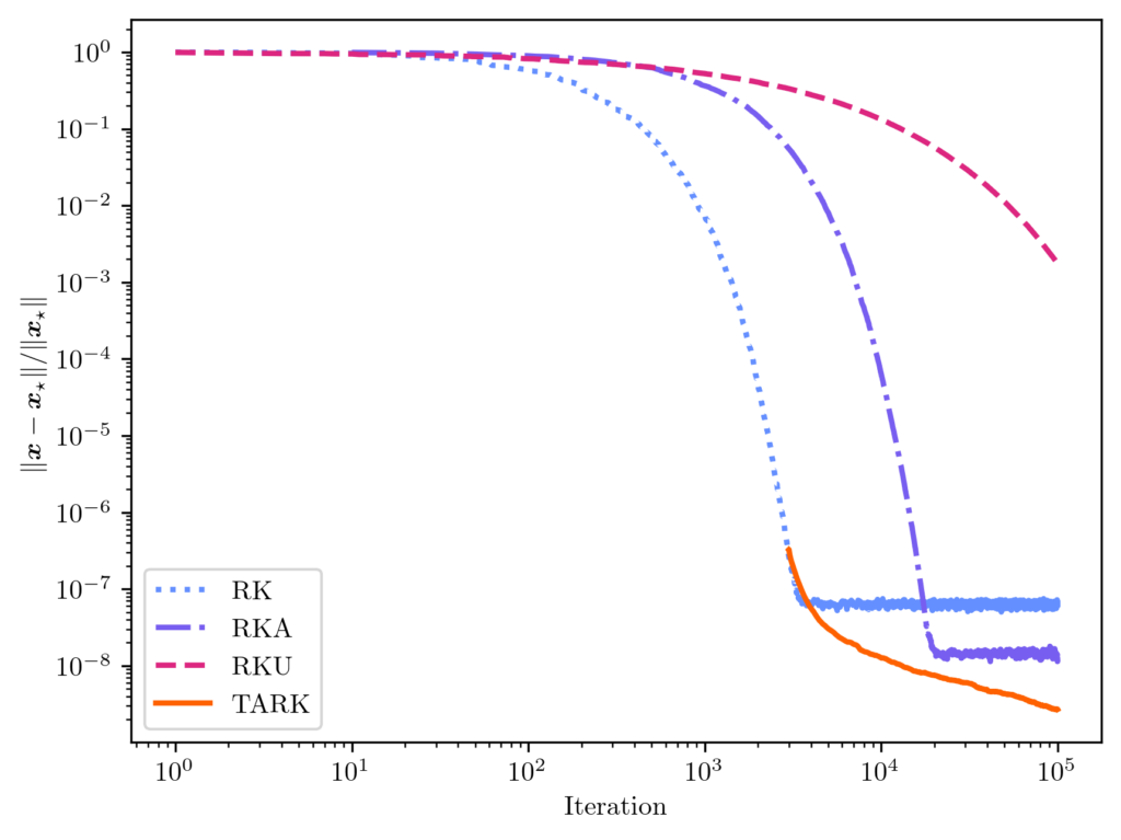
 is the tail-averaged randomized Kaczmarz (TARK) estimator. By Theorem 1, we know the TARK estimator has an exponentially small bias:
 ![\[\norm{\expect[\overline{x}_t] - x_\star} \le (1 - \kappa_{\rm dem}^{-2})^{2(t_{\rm b}+1)} \norm{x_\star}^2.\]](https://www.ethanepperly.com/wp-content/ql-cache/quicklatex.com-89806db87c210bfdd9cbd0e800d65e85_l3.png "Rendered by QuickLaTeX.com")
![\[\expect [\norm{\overline{x}_t - x_\star}^2] \le (1-\kappa_{\rm dem}^{-2})^{t_{\rm b}+1} \norm{x_\star}^2 + \frac{2\kappa_{\rm dem}^4}{t-t_{\rm b}} \frac{\norm{b-Ax_\star}^2}{\norm{A}_{\rm F}^2}.\]](https://www.ethanepperly.com/wp-content/ql-cache/quicklatex.com-d30cb224e4284f0840a46a9757196abf_l3.png "Rendered by QuickLaTeX.com")
 . While the Monte Carlo rate of convergence may be unappealing,
  ;
;  . We found this underrelaxation parameter to lead to a smaller error than the other popular underrelaxation parameter schedule
  .
.
![\[\prob \{ i_t = j \} = \frac{\norm{a_j}^2}{\norm{A}_{\rm F}^2} \eqqcolon p^{\rm RK}_j.\]](https://www.ethanepperly.com/wp-content/ql-cache/quicklatex.com-072dd81a7e854128bf0258a1836003de_l3.png "Rendered by QuickLaTeX.com")
 .
.
 .
. :
: ![\[\prob \{i_t = j\} = p_j.\]](https://www.ethanepperly.com/wp-content/ql-cache/quicklatex.com-95b2f6411ef8d9b8c9b5b61acf6bc928_l3.png "Rendered by QuickLaTeX.com")
![\[D \coloneqq \diag\left( \sqrt{\frac{p_j}{p_j^{\rm RK}}} : j =1,\ldots,n\right).\]](https://www.ethanepperly.com/wp-content/ql-cache/quicklatex.com-bc930770f7b4e20afffe903a4ab372ba_l3.png "Rendered by QuickLaTeX.com")
 is equivalent to the standard RK algorithm run on the diagonally reweighted least-squares problem
 ![\[x_{\rm weighted} = \argmin_{x\in\real^d} \norm{Db-(DA)x}.\]](https://www.ethanepperly.com/wp-content/ql-cache/quicklatex.com-3e1818420a485f35a47361344560d2b1_l3.png "Rendered by QuickLaTeX.com")
 rather than the original least-squares solution
  [mfn}Note that, for this experiment we represent the polynomial
  using its monomial coefficients
  , which has
  equispaced points. We compare the unweighted least-squares solution (orange solid curve) to the weighted least-squares solution using uniform RK weights
  (blue dash-dotted curve). These two curves differ meaningfully, with the weighted least-squares solution having higher error at the ends of the interval but more accuracy in the middle. These differences can be explained looking at the weights (diagonal entries of
  , grey dotted curve), which are lower at the ends of the interval than in the center.
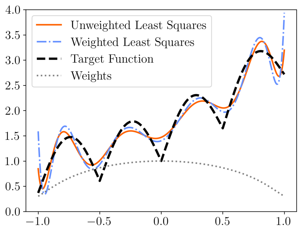
![\[x_{t+1} = \left( I - \frac{a_{i_t}^{\vphantom{\top}}a_{i_t}^\top}{\norm{a_{i_t}}^2} \right)x_t + \frac{b_{i_t}a_{i_t}}{\norm{a_{i_t}}^2}.\]](https://www.ethanepperly.com/wp-content/ql-cache/quicklatex.com-cccfb54762bb990499c96331e7019309_l3.png "Rendered by QuickLaTeX.com")
 denote the
 ![\begin{align*}\expect_{i_t}[x_{t+1}] &= \sum_{j=1}^n \left[\left( I - \frac{a_j^{\vphantom{\top}} a_j^\top}{\norm{a_j}^2} \right)x_t + \frac{b_ja_j}{\norm{a_j}^2}\right] \prob\{i_t=j\}\\ &=\sum_{j=1}^n \left[\left( \frac{\norm{a_j}^2}{\norm{A}_{\rm F}^2}I - \frac{a_j^{\vphantom{\top}} a_j^\top}{\norm{A}_{\rm F}^2} \right)x_t + \frac{b_ja_j}{\norm{A}_{\rm F}^2}\right].\end{align*}](https://www.ethanepperly.com/wp-content/ql-cache/quicklatex.com-0a7f7b3bfad51b7094348db94d2d4254_l3.png "Rendered by QuickLaTeX.com")
 and
and  directly. Therefore, we obtain
 ![\[\expect_{i_t}[x_{t+1}] = \left( I - \frac{A^\top A}{\norm{A}_{\rm F}^2}\right) x_t + \frac{A^\top b}{\norm{A}_{\rm F}^2}.\]](https://www.ethanepperly.com/wp-content/ql-cache/quicklatex.com-de4ded17daf001dde92c26025e9c14f3_l3.png "Rendered by QuickLaTeX.com")
![\[\expect[x_{t+1}] = \left( I - \frac{A^\top A}{\norm{A}_{\rm F}^2}\right) \expect[x_t] + \frac{A^\top b}{\norm{A}_{\rm F}^2}.\]](https://www.ethanepperly.com/wp-content/ql-cache/quicklatex.com-24c5bfe6c1ea70293055deb68a3df117_l3.png "Rendered by QuickLaTeX.com")
 , we obtain
 ![\[\expect[x_t] = \left[\sum_{i=0}^{t-1} \left( I - \frac{A^\top A}{\norm{A}_{\rm F}^2}\right)^i \right]\cdot\frac{A^\top b}{\norm{A}_{\rm F}^2}.\]](https://www.ethanepperly.com/wp-content/ql-cache/quicklatex.com-eb47c96091b1187b53c318589b696693_l3.png "Rendered by QuickLaTeX.com")
![\expect[x_t]](https://www.ethanepperly.com/wp-content/ql-cache/quicklatex.com-fa98c6708608ae4bf5513cf53e74597c_l3.png "Rendered by QuickLaTeX.com") using a matrix
using a matrix  satisfies the formula
 ![\[\sum_{i=0}^\infty y^i = (1-y)^{-1}.\]](https://www.ethanepperly.com/wp-content/ql-cache/quicklatex.com-2d95246c2816e550018d080c58c60240_l3.png "Rendered by QuickLaTeX.com")
 , we get
 ![\[\sum_{i=0}^\infty (1-x)^i = x^{-1}\]](https://www.ethanepperly.com/wp-content/ql-cache/quicklatex.com-726e8fae76877e0ec1f03efab333ec2e_l3.png "Rendered by QuickLaTeX.com")
 . With a little effort, one can check that the same formula
![\[\sum_{i=0}^\infty (I-X)^i = X^{-1}\]](https://www.ethanepperly.com/wp-content/ql-cache/quicklatex.com-1389cddfba9ee14bcbf4293f018c78c9_l3.png "Rendered by QuickLaTeX.com")
 satisfying
  . These conditions hold for the matrix
  since
since ![\[\left(\frac{A^\top A}{\norm{A}_{\rm F}^2}\right)^{-1} = \sum_{i=0}^\infty \left( I - \frac{A^\top A}{\norm{A}_{\rm F}^2}\right)^i. \]](https://www.ethanepperly.com/wp-content/ql-cache/quicklatex.com-8d1be156303c168d2de83dbde76e44d6_l3.png "Rendered by QuickLaTeX.com")
![\[\left(\frac{A^\top A}{\norm{A}_{\rm F}^2}\right)^{-1} = \sum_{i=0}^{t-1} \left( I - \frac{A^\top A}{\norm{A}_{\rm F}^2}\right)^i + \sum_{i=t}^\infty \left( I - \frac{A^\top A}{\norm{A}_{\rm F}^2}\right)^i.\]](https://www.ethanepperly.com/wp-content/ql-cache/quicklatex.com-08f4b1a705439315fe0fc038e059d01c_l3.png "Rendered by QuickLaTeX.com")
 , we obtain
 ![\[\expect[x_t] = x_\star - \left[\sum_{i=t}^\infty \left( I - \frac{A^\top A}{\norm{A}_{\rm F}^2}\right)^i \right]\cdot\frac{A^\top b}{\norm{A}_{\rm F}^2}.\]](https://www.ethanepperly.com/wp-content/ql-cache/quicklatex.com-d973041dba49ba471bbfb6b3d4c2b463_l3.png "Rendered by QuickLaTeX.com")
![\[\expect[x_t] - x_\star = - \left(I - \frac{A^\top A}{\norm{A}_{\rm F}^2}\right)^t \left[\sum_{i=0}^\infty \left( I - \frac{A^\top A}{\norm{A}_{\rm F}^2}\right)^i \right]\cdot\frac{A^\top b}{\norm{A}_{\rm F}^2}.\]](https://www.ethanepperly.com/wp-content/ql-cache/quicklatex.com-8238e65e7b7df2013504f2a6f71799e6_l3.png "Rendered by QuickLaTeX.com")
![\[\expect[x_t] - x_\star = - \left(I - \frac{A^\top A}{\norm{A}_{\rm F}^2}\right)^t x_\star.\]](https://www.ethanepperly.com/wp-content/ql-cache/quicklatex.com-3cbe72663f8ef13c762213b5592bb5d2_l3.png "Rendered by QuickLaTeX.com")
![\[\norm{\expect[x_t] - x_\star}^2 \le \norm{I - \frac{A^\top A}{\norm{A}_{\rm F}^2}}^{2t} \norm{x}_\star^2. \]](https://www.ethanepperly.com/wp-content/ql-cache/quicklatex.com-e663370119bd02900da0aa4f7b6faf03_l3.png "Rendered by QuickLaTeX.com")
 . Let
. Let  be a (
 . Then
 ![\[I - \frac{A^\top A}{\norm{A}_{\rm F}^2} = I - V \cdot\frac{\Sigma^2}{\norm{A}_{\rm F}^2} \cdot V^\top = V \left( I - \frac{\Sigma^2}{\norm{A}_{\rm F}^2}\right)V^\top.\]](https://www.ethanepperly.com/wp-content/ql-cache/quicklatex.com-468566feb9b39f9e0dd616b47f324ad5_l3.png "Rendered by QuickLaTeX.com")
![\[I - \Sigma^2/\norm{A}_{\rm F}^2 = \diag(1 - \sigma^2_{\rm max}(A)/\norm{A}_{\rm F}^2,\ldots,1-\sigma_{\rm min}^2(A)/\norm{A}_{\rm F}^2).\]](https://www.ethanepperly.com/wp-content/ql-cache/quicklatex.com-4bc7dac794d8913157b82fd0df23e41d_l3.png "Rendered by QuickLaTeX.com")
 . We have invoked the definition of the Demmel condition number (2). Therefore, plugging into (7), we obtain
 ![\[\norm{\expect[x_t] - x_\star}^2 \le \left(1-\kappa_{\rm dem}^{-2}\right)^{2t} \norm{x}_\star^2,\]](https://www.ethanepperly.com/wp-content/ql-cache/quicklatex.com-7c29ce0386ec23c163afab561f181af1_l3.png "Rendered by QuickLaTeX.com")
 an
an  ?
? . Throughout this post, I will assume knowledge of sketching; see my previous
  , and these parameters are related
  .
.![\[\expect\Big[\big((SA)^\top (SA)\big)^{-1}\Big] \ne \big(A^\top A\big)^{-1}\]](https://www.ethanepperly.com/wp-content/ql-cache/quicklatex.com-0cd441af1378414d36a71a4405630eab_l3.png "Rendered by QuickLaTeX.com")
 . The sketch-and-solve solution
  does not change under a scaling of the matrix
 ![\[S \in \real^{\ell\times n} \quad \text{with } S_{ij} \sim \text{Normal}(0,1) \text{ iid},\]](https://www.ethanepperly.com/wp-content/ql-cache/quicklatex.com-4241ac9b0c6ffe780ecf8f59abbb6f2e_l3.png "Rendered by QuickLaTeX.com")
 be a full column-rank matrix. Then
 ![\[\expect[(SA)^\dagger(Sb)] = A^\dagger b. \]](https://www.ethanepperly.com/wp-content/ql-cache/quicklatex.com-6c135e0524dca0ed8d764479c79be876_l3.png "Rendered by QuickLaTeX.com")
 is an unbiased estimate for the least-squares solution
  .
.
![\[A^\dagger b = \operatorname*{argmin}_{x\in\real^d} \norm{Ax - b}.\]](https://www.ethanepperly.com/wp-content/ql-cache/quicklatex.com-758a2563a025ea5eb02093ee09e269a2_l3.png "Rendered by QuickLaTeX.com")
![\[A^\dagger = (A^\top A)^{-1} A^\top,\]](https://www.ethanepperly.com/wp-content/ql-cache/quicklatex.com-54e18e841ca1d2908256c65ccb31637f_l3.png "Rendered by QuickLaTeX.com")
 has the same distribution as
 ![\[A = U\twobyone{\Sigma}{0}V^\top\]](https://www.ethanepperly.com/wp-content/ql-cache/quicklatex.com-b86bfeff6ec3786014519ea5b890b2b4_l3.png "Rendered by QuickLaTeX.com")
![\[A \mapsto U^\top A V, \quad S \mapsto V^\top SU, \quad b \mapsto U^\top b.\]](https://www.ethanepperly.com/wp-content/ql-cache/quicklatex.com-77b2e6a2a41be700f4503e57299c9dfb_l3.png "Rendered by QuickLaTeX.com")
![\[A = \twobyone{\Sigma}{0}.\]](https://www.ethanepperly.com/wp-content/ql-cache/quicklatex.com-662c1bf602a21154cf1e5355e6fdc115_l3.png "Rendered by QuickLaTeX.com")
![\[b = \twobyone{b_1}{b_2}, \quad S = \onebytwo{S_1}{S_2}.\]](https://www.ethanepperly.com/wp-content/ql-cache/quicklatex.com-27fd1fd3e8f3f44834436bb2110fd7ba_l3.png "Rendered by QuickLaTeX.com")
![\[A^\dagger b = \Sigma^{-1}b_1.\]](https://www.ethanepperly.com/wp-content/ql-cache/quicklatex.com-b23ab2580fa2fdad9fcfddf3df225fbd_l3.png "Rendered by QuickLaTeX.com")
 . Begin by using the normal equations (4) to write out the sketch-and-solve solution
 ![\[(SA)^\dagger (Sb) = [(SA)^\top (SA)]^{-1}(SA)^\top (Sb).\]](https://www.ethanepperly.com/wp-content/ql-cache/quicklatex.com-52c84e0a183fe2e46f36f62446379edb_l3.png "Rendered by QuickLaTeX.com")
![\[(SA)^\dagger (Sb) = [\Sigma S_1^\top S_1\Sigma]^{-1}\Sigma S_1^\top \onebytwo{S_1}{S_2}\twobyone{b_1}{b_2}.\]](https://www.ethanepperly.com/wp-content/ql-cache/quicklatex.com-2800b69708b037d55eeeb98fa104dd82_l3.png "Rendered by QuickLaTeX.com")
![\[(SA)^\dagger (Sb) = \Sigma^{-1}(S_1^\top S_1)^{-1} S_1^\top (S_1b_1 + S_2 b_2).\]](https://www.ethanepperly.com/wp-content/ql-cache/quicklatex.com-3f4f56224702b904c6bf72d965d20386_l3.png "Rendered by QuickLaTeX.com")
![\[(SA)^\dagger (Sb) = \Sigma^{-1}b_1 + \Sigma^{-1} S_1^\dagger S_2b_2 = A^\dagger b + \Sigma^{-1} S_1^\dagger S_2b_2. \]](https://www.ethanepperly.com/wp-content/ql-cache/quicklatex.com-49f9435ad832dcae09cd3344a01c4b3e_l3.png "Rendered by QuickLaTeX.com")
 and
and  are independent and
 ![\expect[S_2] = 0](https://www.ethanepperly.com/wp-content/ql-cache/quicklatex.com-57f5284f6ae7b9df499d484d49926dae_l3.png "Rendered by QuickLaTeX.com") . Thus, taking expectations, we obtain
. Thus, taking expectations, we obtain![\[\expect[(SA)^\dagger (Sb)] = A^\dagger b + \Sigma^{-1} \expect[S_1^\dagger] \expect[S_2]b_2 = A^\dagger b.\]](https://www.ethanepperly.com/wp-content/ql-cache/quicklatex.com-f45600345d37f0812e850b8c1a16e030_l3.png "Rendered by QuickLaTeX.com")
 columns of
  columns of
 ![\[\expect \norm{A\hat{x} - b}^2,\]](https://www.ethanepperly.com/wp-content/ql-cache/quicklatex.com-b66ecc55bd4f68677bc892deded4ed12_l3.png "Rendered by QuickLaTeX.com")
 is the sketch-and-solve solution. We write the expected residual norm as
 ![\[\expect\norm{A\hat{x} - b}^2 = \expect\norm{\twobyone{b_1 + S_1^\dagger S_2b_2}{0} - \twobyone{b_1}{b_2}}^2 = \norm{b_2}^2 + \expect\norm{S_1^\dagger S_2b_2}^2.\]](https://www.ethanepperly.com/wp-content/ql-cache/quicklatex.com-a7dce4f3a10550b2a4c1b24039097db8_l3.png "Rendered by QuickLaTeX.com")
![\[\expect\norm{A\hat{x} - b}^2 = \left(1+\frac{d}{\ell-d-1}\right)\norm{b_2}^2.\]](https://www.ethanepperly.com/wp-content/ql-cache/quicklatex.com-5fffa05a8417a7fa7a7c51d53c765f5f_l3.png "Rendered by QuickLaTeX.com")
 is the optimal least-squares residual
  . Thus, we have shown
 ![\[\expect\norm{A\hat{x} - b}^2 = \left(1+\frac{d}{\ell-d-1}\right)\min_{x\in\real^d} \norm{Ax-b}^2.\]](https://www.ethanepperly.com/wp-content/ql-cache/quicklatex.com-0aa56378e18dd3b779e91d08c25c07e3_l3.png "Rendered by QuickLaTeX.com")
 larger than the optimal value. In particular,
 ![\[\expect\norm{A\hat{x} - b}^2 = \left(1+\varepsilon\right)\min_{x\in\real^d} \norm{Ax-b}^2 \quad \text{when } \ell = \frac{d}{\varepsilon} + d + 1.\]](https://www.ethanepperly.com/wp-content/ql-cache/quicklatex.com-423a327d2db81e2aed6aa072386518a2_l3.png "Rendered by QuickLaTeX.com")
 be random vectors in
  drawn uniformly at random from the sphere of radius
  ,
, -dimensional
 ![\[q \coloneqq x^\top Ax\]](https://www.ethanepperly.com/wp-content/ql-cache/quicklatex.com-2335446c01894126b9be9427e85de438_l3.png "Rendered by QuickLaTeX.com")
![\[\hat{\tr}\coloneqq \frac{1}{m}\sum_{i=1}^m x_i^\top Ax_i.\]](https://www.ethanepperly.com/wp-content/ql-cache/quicklatex.com-f3db7ad20e68a6a0d6089c98794613f1_l3.png "Rendered by QuickLaTeX.com")
 are unbiased estimates for the trace of
 ![\expect[q] = \expect[\hat{\tr}] = \tr A](https://www.ethanepperly.com/wp-content/ql-cache/quicklatex.com-41d88b5cbaa2e924f0d83e85fd3d76e8_l3.png "Rendered by QuickLaTeX.com") . The goal of this post will be to bound the probability of these quantities being much smaller or larger than the trace of
. The goal of this post will be to bound the probability of these quantities being much smaller or larger than the trace of  independent copies of the random variable
 ![\[\overline{A} = A - \frac{\tr A}{n}I.\]](https://www.ethanepperly.com/wp-content/ql-cache/quicklatex.com-bd4e8dbd667c23444824ae5ce6aa8db4_l3.png "Rendered by QuickLaTeX.com")
 has the effect of shifting
  has trace zero.
![\[q = x^\top A x = x^\top \overline{A} x + \frac{\tr A}{n} \cdot x^\top I x = x^\top \overline{A} x + \tr A.\]](https://www.ethanepperly.com/wp-content/ql-cache/quicklatex.com-3bcc2b942b5442a19b03b3b012fbfedb_l3.png "Rendered by QuickLaTeX.com")
 . Rearranging, we see that the error
  satisfies
![\[\overline{q} = q-\tr A = x^\top \overline{A}x.\]](https://www.ethanepperly.com/wp-content/ql-cache/quicklatex.com-d2c3289e2fa1a4a5a59762b69593fcb1_l3.png "Rendered by QuickLaTeX.com")
 depends only on the centered matrix
  , and the
  . These observations will be important later.
 , define the cumulant generating function (cgf)
 ![\[\xi_z(\theta) = \log (\expect [\exp(\theta z)]).\]](https://www.ethanepperly.com/wp-content/ql-cache/quicklatex.com-75f376a73cb1e931a07fb50331747dcb_l3.png "Rendered by QuickLaTeX.com")
 is a vector with
  , where
  is a scaling factor.
 is a
is a 
 degrees of freedom.
![\expect[a^2] = 1](https://www.ethanepperly.com/wp-content/ql-cache/quicklatex.com-5a29d04b84a1f93ace9e404ce3616f54_l3.png "Rendered by QuickLaTeX.com") .
.![\expect[\norm{g}^2] = \sum_{i=1}^n \expect[g_i^2] = n](https://www.ethanepperly.com/wp-content/ql-cache/quicklatex.com-454dd5415485ca62bb66120b18283c66_l3.png "Rendered by QuickLaTeX.com") . But also,
. But also, ![\expect[\norm{g}^2] = \expect[a^2] \cdot \expect[\norm{x}^2] = \expect[a^2] \cdot n](https://www.ethanepperly.com/wp-content/ql-cache/quicklatex.com-f153f4a0af6e2dd00a85f40f2ff2fca8_l3.png "Rendered by QuickLaTeX.com") . Therefore,
. Therefore, ![\expect[a^2]=1](https://www.ethanepperly.com/wp-content/ql-cache/quicklatex.com-0bd7a7c95fafaa9724e054eb87cba203_l3.png "Rendered by QuickLaTeX.com") .
.![\[g^\top \overline{A} g = a^2 \cdot x^\top \overline{A} x = a^2 \cdot \overline{q}.\]](https://www.ethanepperly.com/wp-content/ql-cache/quicklatex.com-5e24054c3179f84adac8e8f2c69d1514_l3.png "Rendered by QuickLaTeX.com")
![\[\xi_{\overline{q}}(\theta) \le \xi_{g^\top A g}(\theta) \quad \text{for all } \theta \in \real.\]](https://www.ethanepperly.com/wp-content/ql-cache/quicklatex.com-34b5802e38a63f46468b24fbd0108a08_l3.png "Rendered by QuickLaTeX.com")
![\[\xi_{z}(\theta) \le \xi_{bz}(\theta) \quad \text{for all } \theta \in \real.\]](https://www.ethanepperly.com/wp-content/ql-cache/quicklatex.com-634696ad9a505fc68c577e80323c4324_l3.png "Rendered by QuickLaTeX.com")
 and
and  denote expectations take over the randomness in
 ![\expect[\cdot] = \expect_z[\expect_b[\cdot ]]](https://www.ethanepperly.com/wp-content/ql-cache/quicklatex.com-332d248f563a792e91ea931b068aa939_l3.png "Rendered by QuickLaTeX.com") . Begin with the right-hand side and invoke
. Begin with the right-hand side and invoke ![\[\xi_{bz}(\theta) = \xi_z(\theta) = \log (\expect_z [\expect_b [\exp(\theta bz)]]) \ge \log (\expect_z [\exp(\theta \expect_b[b]z)]) = \xi_z(\theta).\]](https://www.ethanepperly.com/wp-content/ql-cache/quicklatex.com-fa5226c666db21a3f56f6bdfdcbb1170_l3.png "Rendered by QuickLaTeX.com")
![\expect[b] = 1](https://www.ethanepperly.com/wp-content/ql-cache/quicklatex.com-bb25ca2a980b2795822bf62c2d392b47_l3.png "Rendered by QuickLaTeX.com") and the definition of the cgf.
and the definition of the cgf.
 for all
  .
. for a trace-zero matrix
 ![\[\xi_{\overline{q}}(\theta) \le \xi_{g^\top \overline{A} g}(\theta) \le \frac{\theta^2 \norm{\overline{A}}_{\rm F}^2}{1 - 2\theta \norm{\overline{A}}}.\]](https://www.ethanepperly.com/wp-content/ql-cache/quicklatex.com-623e28881a1cb46a4526687b07e28e0e_l3.png "Rendered by QuickLaTeX.com")
![\[\prob \{ x^\top A x - \tr(A) \ge t \} \le \exp \left( - \frac{t^2/2}{2 \norm{\overline{A}}_{\rm F}^2 + 2 \overline{\norm{\overline{A}}t}} \right).\]](https://www.ethanepperly.com/wp-content/ql-cache/quicklatex.com-16071627e38437191476b04f643b1057_l3.png "Rendered by QuickLaTeX.com")
 by instantiating this result with
  .
. ![\[\prob \{ |x^\top A x - \tr(A)| \ge t \} \le 2\exp \left( - \frac{t^2/2}{2 \norm{\overline{A}}_{\rm F}^2 + 2 \overline{\norm{\overline{A}}t}} \right).\]](https://www.ethanepperly.com/wp-content/ql-cache/quicklatex.com-f19454359ca5d0e68b0207b865db95db_l3.png "Rendered by QuickLaTeX.com")
 or
or  are known as
  for small
  for large
  . This pattern of results “subgaussian scaling for small
 ![\[\prob \{ g^\top A g - \tr A \ge t \} \le \exp \left( -\frac{t^2/2}{C\norm{A}_{\rm F}^2 + c t \norm{A}}\right)\]](https://www.ethanepperly.com/wp-content/ql-cache/quicklatex.com-cb3646b736a9e33403f0175d6bc8e296_l3.png "Rendered by QuickLaTeX.com")
 . For vectors on the sphere,
  and
and  have been replaced by
  and
and  which are always smaller (and sometimes much smaller). The smaller tail probabilities for
  . For small
  . The true variance of
  is
is ![\[\Var(q) = \frac{n}{n+2} \cdot 2\norm{\overline{A}}_{\rm F}^2,\]](https://www.ethanepperly.com/wp-content/ql-cache/quicklatex.com-350430c2a39ce9f557afb3d41806c93f_l3.png "Rendered by QuickLaTeX.com")
 easily follow. Indeed, the cgf is additive for independent random variables and satisfies the identity
  for constant $c, so
 ![\[\xi_{\overline{\tr}}(\theta) = \sum_{i=1}^m \xi_{x_i^\top Ax_i}(\theta/m) \le m \cdot \frac{(\theta/m)^2 \norm{\overline{A}}_{\rm F}^2}{1 - 2(\theta/m)\norm{\overline{A}}}.\]](https://www.ethanepperly.com/wp-content/ql-cache/quicklatex.com-d6d7f289a105bd06e272223f56ee7080_l3.png "Rendered by QuickLaTeX.com")

 is a vector. For simplicity, we assume that this system is
  , randomized Kaczmarz repeatedly performs the following steps:
 . Here, and going forward,
  denotes the
  th row of
  is the
  .
. and compute their norms
  . Then, sampling can be done using any algorithm for sampling from a weighted list of items. But what if
 ![\[\norm{a_i}^2 \le B \quad \text{for each } i = 1,\ldots,n.\]](https://www.ethanepperly.com/wp-content/ql-cache/quicklatex.com-a80c9da38c2d98b188cb70f64c8637e8_l3.png "Rendered by QuickLaTeX.com")
![[-1,1]](https://www.ethanepperly.com/wp-content/ql-cache/quicklatex.com-634fe4705a526f221e312cffd3ceda93_l3.png "Rendered by QuickLaTeX.com") , then (1) holds with
, then (1) holds with  . To sample a row
  , we perform the following the rejection sampling procedure:
 uniformly at random (i.e.,
  is equally likely to be any row index between
  , accept and set
  . With the remaining probability
  , reject and return to step 1.
 . Our goal is to choose a random index
  , i.e.,
  . We will call
  the target distribution. (Note that we do not require the weights
  .)
.) . Further, suppose that the proposal distribution dominates the target distribution in the sense that
 ![\[w_i \le \rho_i \quad \text{for each } i=1,\ldots,n.\]](https://www.ethanepperly.com/wp-content/ql-cache/quicklatex.com-7f2901cd8e565853465062e41a59b5bd_l3.png "Rendered by QuickLaTeX.com")
 , accept and set
  and
and  for all
  , after which the probability of accepting
  . Therefore, the probability of outputting
 ![\[\prob \{\text{$i$ accepted this loop}\} = \frac{\rho_i}{\sum_{j=1}^n \rho_j} \cdot \frac{w_i}{\rho_i} = \frac{w_i}{\sum_{j=1}^n \rho_j}.\]](https://www.ethanepperly.com/wp-content/ql-cache/quicklatex.com-f8fb5712ddc38527600d4fd51394bfc7_l3.png "Rendered by QuickLaTeX.com")
![\[\prob \{\text{any accepted this loop}\} = \sum_{i=1}^n \prob \{\text{$i$ accepted this loop}\} = \frac{\sum_{i=1}^n w_i}{\sum_{i=1}^n \rho_i}.\]](https://www.ethanepperly.com/wp-content/ql-cache/quicklatex.com-87004ae4b99269f6917de03d3a4ec86e_l3.png "Rendered by QuickLaTeX.com")
![\[\prob \{\text{$i$ accepted this loop} \mid \text{any accepted this loop}\} = \frac{\prob \{\text{$i$ accepted this loop}\}}{\prob \{\text{any accepted this loop}\}} = \frac{w_i}{\sum_{j=1}^n w_j}.\]](https://www.ethanepperly.com/wp-content/ql-cache/quicklatex.com-8740003cf2cc5dfd18def3387663bcc2_l3.png "Rendered by QuickLaTeX.com")
 , the ratio of the total mass of the target
  . Thus, rejection sampling will have a high acceptance rate if
  and a low acceptance rate if
  . The conclusion for practice is that rejection sampling is only computationally efficient if one has access to a good proposal distribution
  .
. , but this not all that rejection sampling can do. Indeed, one can also use rejection sampling for sampling a real-valued parameters
  or a multivariate parameter
  and
and  are necessary to define the sampling probabilities
  and
and  , as computing
  denote the initial matrix and
  denote a trivial initial approximation. For
  , RPCholesky performs the following steps:
 with probability
  .
. . Here,
  denotes the
  .
. .
. . With an optimized implementation, RPCholesky requires only
  operations and evaluates just
 denote the first
  produced by
 ![\[\hat{A}^{(j)} = A(:,S_j) A(S_j,S_j)^{-1}A(S_j,:). \]](https://www.ethanepperly.com/wp-content/ql-cache/quicklatex.com-ebc63948bd7d20eda4ccafa74555ba6b_l3.png "Rendered by QuickLaTeX.com")
![\[A^{(j)} = A - \hat{A}^{(j)} = A - A(:,S_j) A(S_j,S_j)^{-1}A(S_j,:).\]](https://www.ethanepperly.com/wp-content/ql-cache/quicklatex.com-dc5136dd307c099cb5fa70663104166b_l3.png "Rendered by QuickLaTeX.com")
![\[A^{(j)}_{ii} = A_{ii} - A(i,S_j) A(S_j,S_j)^{-1} A(S_j,i).\]](https://www.ethanepperly.com/wp-content/ql-cache/quicklatex.com-f8442521e6a6003a935f35d25aca1c73_l3.png "Rendered by QuickLaTeX.com")
 is cheap, just requiring some arithmetic involving matrices and vectors of size
  , but it is expensive to evaluate all of the
  . (One may verify that, as required,
  for all
  , sample random indices
  using rejection sampling with proposal distribution
  are evaluated on an as-needed basis using (2).
 and
and  . The first matrix
  to its
  . The other matrix
  . Let’s see how long it takes to compute their eigenvalue decompositions in MATLAB:
 longer to compute the eigenvalues of the non-Hermitian matrix
  of eigenvectors for a Hermitian matrix
  is a
is a  .
. . The matrix
  of eigenvectors for a normal matrix
  is also unitary,
  . An important class of normal matrices are unitary matrices themselves. A unitary matrix
  .
.![\[C = H + iS, \quad H = \frac{C+C^*}{2}, \quad S = \frac{C-C^*}{2i}.\]](https://www.ethanepperly.com/wp-content/ql-cache/quicklatex.com-5efdc333ce38cd9aaa9c5c10ad40b44a_l3.png "Rendered by QuickLaTeX.com")
 . We know from matrix theory that commuting Hermitian matrices are
  and
and  for diagonal matrices
  and
and  . Thus, given access to such
 ![\[C = Q(D_H+iD_S)Q^*.\]](https://www.ethanepperly.com/wp-content/ql-cache/quicklatex.com-d84fd3e79327e2e4082ba99967de3c9e_l3.png "Rendered by QuickLaTeX.com")
 for this matrix has a repeated eigenvalue. Thus,
  of the Hermitian and skew-Hermitian parts of
  and
and  .
. .
. unitary matrix, RandDiag takes 0.4 seconds, just as fast as the Hermitian eigendecomposition did.
 , a matrix
  will also diagonalize
  . But, for any specific choice of
  , there is a possibility of failure. To avoid this possibility, we can just pick
  and
and  at random. It’s really as simple as that.
 with
with  , its (
 , where
  is a
is a  is
is  test matrix. It takes about 2.5 seconds to run.
 is the
  is also small:
 , computing its (upper triangular)
  , and setting
  . Cholesky QR is very fast, about
  faster than Householder QR for this example:
 , about ten million times larger than for Householder QR!:
 . The condition number of
  , which is at the root of Cholesky QR’s loss of accuracy. Thus, Cholesky QR is only appropriate for matrices that are well-conditioned, having a small condition number
  , say
, say  .
. that
that  is well-conditioned. Then, since
  ; see
; see  . This step compresses the very tall matrix
  to the much shorter matrix
  .
. using Householder QR. Since the matrix
  .
. . Observe that
  , as desired.
 faster in our experiment:
 by a change of variables,
  .
. . This result is just duality for the
  norm.
norm. Taking
  for
for  to be each of the
  of an
of an  matrix
  . The classical method for this purpose is the
 ![\[\hat{\tr} = \frac{1}{m} \left( x_1^\top Ax_1 + \cdots + x_m^\top Ax_m \right),\]](https://www.ethanepperly.com/wp-content/ql-cache/quicklatex.com-f27a0c05da428b96172a0a8ab23ca54b_l3.png "Rendered by QuickLaTeX.com")
 are
are ![\[\expect[x_ix_i^\top] = I.\]](https://www.ethanepperly.com/wp-content/ql-cache/quicklatex.com-b5ac53011350edc256d9b8c66fdbe7c8_l3.png "Rendered by QuickLaTeX.com")
 with equal probabilities (i.e.,
  .
.![\expect[\hat{\tr}] = \tr(A)](https://www.ethanepperly.com/wp-content/ql-cache/quicklatex.com-ad9e9d417b59555f2a6e78e78b6bcbe9_l3.png "Rendered by QuickLaTeX.com") , the
, the  of the Girard–Hutchinson estimator with different choices of test vectors. In that post, I stated the formulas for different choices of test vectors (Gaussian, random signs, sphere) and showed how those formulas could be proven.
 be the
 ![\[\overline{\lambda} = \frac{\lambda_1 + \cdots + \lambda_n}{n}.\]](https://www.ethanepperly.com/wp-content/ql-cache/quicklatex.com-3f9e9cf25f6cf20463de5be7e8d40f88_l3.png "Rendered by QuickLaTeX.com")
![\[\Var(\hat{\tr}_{\rm Gaussian}) = \frac{1}{m} \cdot 2 \sum_{i=1}^n \lambda_i^2.\]](https://www.ethanepperly.com/wp-content/ql-cache/quicklatex.com-f8dc441dc68294b0d6ff6af42d3ecef5_l3.png "Rendered by QuickLaTeX.com")
![\[\Var(\hat{\tr}_{\rm sphere}) = \frac{1}{m} \cdot \frac{n}{n+2} \cdot 2\sum_{i=1}^n (\lambda_i - \overline{\lambda})^2.\]](https://www.ethanepperly.com/wp-content/ql-cache/quicklatex.com-6a275f8ba8a47be085e22f679b60b497_l3.png "Rendered by QuickLaTeX.com")
 is smaller than
  by a factor of
  . This improvement is quite minor. Second, and more importantly,
  and
and  with a (
 , we take
  . Below show the variance of Girard–Hutchinson estimator for different distributions for the test vector. We see that the sphere distribution leads to a trace estimate which has a variance 300× smaller than the Gaussian distribution. For this example, the sphere and random sign distributions are similar.
 )
)

![\[\Var(\hat{\tr}_{\rm signs}) = 2 \sum_{i\ne j} A_{ij}^2.\]](https://www.ethanepperly.com/wp-content/ql-cache/quicklatex.com-3a6665f8e55563640aedd5ebb0945409_l3.png "Rendered by QuickLaTeX.com")
 depends on the size of the off-diagonal entries of