Which Sketch Should I Use? – Ethan N. Epperly

This is the second of a sequence of two posts on sketching, which I’m doing on the occasion of my new paper on the numerical stability of the iterative sketching method. For more on what sketching is and how it can be used to solve computational problems, I encourage you to check out the first post.

The goals of this post are more narrow. I seek to answer the question:

Which sketching matrix should I use?

To cut to the chase, my answer to this question is:

Sparse sign embeddings are a sensible default for sketching.

There are certainly cases when sparse sign embeddings are not the best type of sketch to use, but I hope to convince you that they’re a good sketching matrix to use for most purposes.

Experiments

Let’s start things off with some numerical experiments.¹ We’ll compare three types of sketching matrices: Gaussian embeddings, a subsampled randomized trigonometric transform (SRTT), and sparse sign embeddings. See the last post for descriptions of these sketching matrices. I’ll discuss a few additional types of sketching matrices that require more discussion at the end of this post.

Recall that a sketching matrix $S \in \real^{d\times n}$ seeks to compress a high-dimensional matrix $A \in \real^{n\times k}$ or vector $b\in\real^n$ to a lower-dimensional sketched matrix $SA$ or vector $Sb$ . The quality of a sketching matrix for a matrix $A$ is measured by its distortion $\varepsilon$ , defined to be the smallest number $\varepsilon > 0$ such that

$(1-\varepsilon) \norm{x} \le \norm{Sx} \le (1+\varepsilon) \norm{x} \quad \text{for every } x \in \operatorname{col}(A).$

Here, $\operatorname{col}(A)$ denotes the column space of the matrix $A$ .

Timing

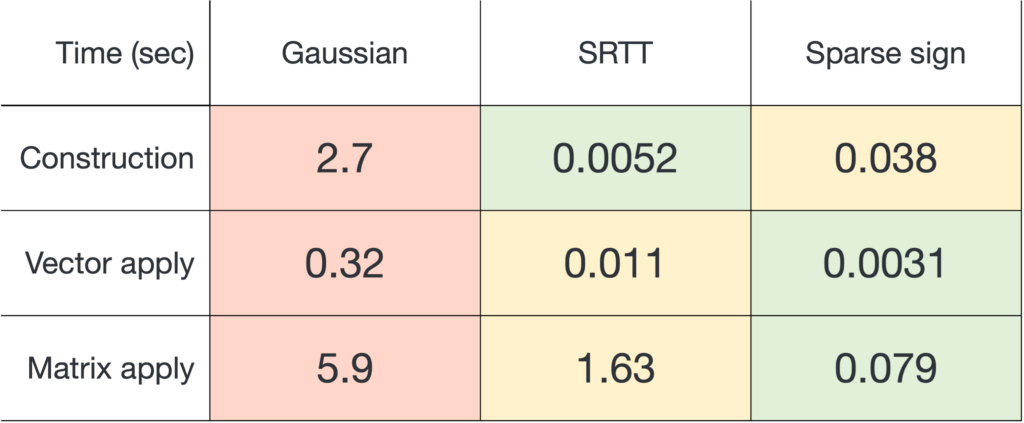
We begin with timing test. We will measure three different times for each embedding:

Construction. The time required to generate the sketching matrix $S$ .
Vector apply. The time to apply the sketch to a single vector.
Matrix apply. The time to apply the sketch to an $n\times 200$ matrix.

We will test with input dimension $n = 10^6$ (one million) and output dimension $d = 400$ . For the SRTT, we use the discrete cosine transform as our trigonometric transform. For the sparse sign embedding, we use a sparsity parameter $\zeta = 8$ .

Here are the results (timings averaged over 20 trials):

Our conclusions are as follows:

Sparse sign embeddings are definitively the fastest to apply, being 3–20× faster than the SRTT and 74–100× faster than Gaussian embeddings.
Sparse sign embeddings are modestly slower to construct than the SRTT, but much faster to construct than Gaussian embeddings.

Overall, the conclusion is that sparse sign embeddings are the fastest sketching matrices by a wide margin: For an “end-to-end” workflow involving generating the sketching matrix $S \in \real^{400\times 10^6}$ and applying it to a matrix $A\in\real^{10^6\times 200}$ , sparse sign embeddings are 14× faster than SRTTs and 73× faster than Gaussian embeddings.²

Distortion

Runtime is only one measure of the quality of a sketching matrix; we also must care about the distortion $\varepsilon$ . Fortunately, for practical purposes, Gaussian embeddings, SRTTs, and sparse sign embeddings all tend to have similar distortions. Therefore, we are free to use the sparse sign embeddings, as they as typically are the fastest.

Consider the following test. We generate a sparse random test matrix $A$ of size $n\times k$ for $n = 10^5$ and $k = 50$ using the MATLAB sprand function; we set the sparsity level to 1%. We then compare the distortion of Gaussian embeddings, SRTTs, and sparse sign embeddings across a range of sketching dimensions $d$ between 100 and 10,000. We report the distortion averaged over 100 trials. The theoretically predicted value $\varepsilon = \sqrt{k/d}$ (equivalently, $d=k/\varepsilon^2$ ) is shown as a dashed line.

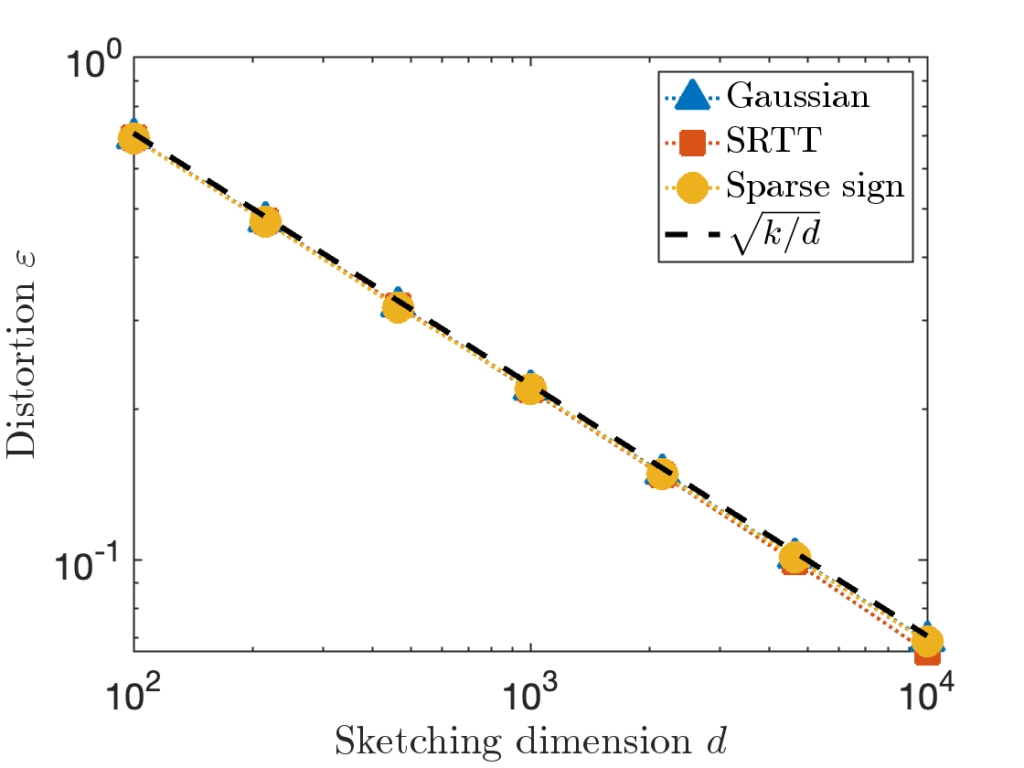
To me, I find these results remarkable. All three embeddings exhibit essentially the same distortion parameter predicted by the Gaussian theory.

It would be premature to declare success having only tested on one type of test matrix $A$ . Consider the following four test matrices:

Sparse: The test matrix from above.
Dense: $A\in\real^{10^6\times 50}$ is taken to be a matrix with independent standard Gaussian random values.
Khatri–Rao: $A\in\real^{50^3\times 50}$ is taken to be the Khatri–Rao product of three Haar random orthogonal matrices.
Identity: $A = \twobyone{I}{0} \in\real^{10^6\times 50}$ is taken to be the $50\times 50$ identity matrix stacked onto a $(10^6-50)\times 50$ matrix of zeros.

The performance of sparse sign embeddings (again with sparsity parameter $\zeta = 8$ ) is shown below:

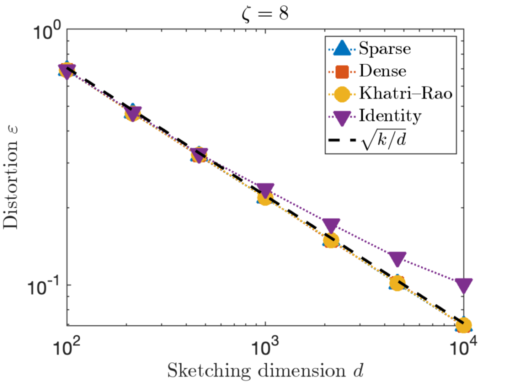
We see that for the first three test matrices, the performance closely follows the expected value $\epsilon = \sqrt{k/d}$ . However, for the last test matrix “Identity”, we see the distortion begins to slightly exceed this predicted distortion for $d/k\ge 20$ .

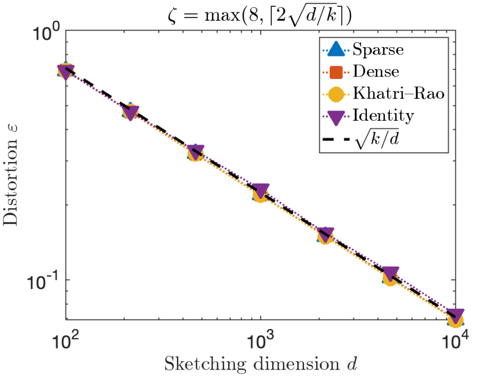
To improve sparse sign embeddings for higher values of $d/k$ , we can increase the value of the sparsity parameter $\zeta$ . We recommend

$\zeta = \max \left( 8 , \left\lceil 2\sqrt{\frac{d}{k}} \right\rceil \right).$

With this higher sparsity level, the distortion closely tracks $\varepsilon = \sqrt{k/d}$ for all four test matrices:

Conclusion

Implemented appropriately (see below), sparse sign embeddings can be faster than other sketching matrices by a wide margin. The parameter choice $\zeta = 8$ is enough to ensure the distortion closely tracks $\varepsilon = \sqrt{k/d}$ for most test matrices. For the toughest test matrices, a slightly larger sparsity parameter $\zeta = \max(8, \lceil 2\sqrt{d/k}\rceil)$ can be necessary to achieve the optimal distortion.

While these tests are far from comprehensive, they are consistent with the uniformly positive results for sparse sign embeddings reported in the literature. We believe that this evidence supports the argument that sparse sign embeddings are a sensible default sketching matrix for most purposes.

Sparse Sign Embeddings: Theory and Practice

Given the highly appealing performance characteristics of sparse sign embeddings, it is worth saying a few more words about these embeddings and how they perform in both theory and practice.

Recall that a sparse sign embedding is a random matrix of the form

$S = \frac{1}{\sqrt{\zeta}} \begin{bmatrix} s_1 & \cdots & s_n \end{bmatrix}.$

Each column $s_i$ is an independent and randomly generated to contain exactly $\zeta$ nonzero entries in uniformly random positions. The value of each nonzero entry of $s_i$ is chosen to be either $+1$ or $-1$ with 50/50 odds.

Parameter Choices

The goal of sketching is to reduce vectors of length $n$ to a smaller dimension $d$ . For linear algebra applications, we typically want to preserve all vectors in the column space of a matrix $A$ up to distortion $\varepsilon > 0$ :

$(1-\varepsilon) \norm{x} \le \norm{Sx} \le (1+\varepsilon) \norm{x} \quad \text{for all }x \in \operatorname{col}(A).$

To use sparse sign embeddings, we must choose the parameters appropriately:

Given a dimension $k$ and a target distortion $\varepsilon$ , how do we pick $d$ and $\zeta$ ?

Based on the experiments above (and other testing reported in the literature), we recommend the following parameter choices in practice:

$d = \frac{k}{\varepsilon^2} \quad \text{and} \quad \zeta = \max\left(8,\frac{2}{\varepsilon}\right).$

The parameter choice $\zeta = 8$ is advocated by Tropp, Yurtever, Udell, and Cevher; they mention experimenting with parameter values as small as $\zeta = 2$ . The value $\zeta = 1$ has demonstrated deficiencies and should almost always be avoided (see below). The scaling $d \approx k/\varepsilon^2$ is derived from the analysis of Gaussian embeddings. As Martinsson and Tropp argue, the analysis of Gaussian embeddings tends to be reasonably descriptive of other well-designed random embeddings.

The best-known theoretical analysis, due to Cohen, suggests more cautious parameter setting for sparse sign embeddings:

$d = \mathcal{O} \left( \frac{k \log k}{\varepsilon^2} \right) \quad \text{and} \quad \zeta = \mathcal{O}\left( \frac{\log k}{\varepsilon} \right).$

The main difference between Cohen’s analysis and the parameter recommendations above is the presence of the $\log k$ factor and the lack of explicit constants in the O-notation.

Implementation

For good performance, it is imperative to store $S$ using either a purpose-built data structure or a sparse matrix format (such as a MATLAB sparse matrix or scipy sparse array).

If a sparse matrix library is unavailable, then either pursue a dedicated implementation or use a different type of embedding; sparse sign embeddings are just as slow as Gaussian embeddings if they are stored in an ordinary non-sparse matrix format!

Even with a sparse matrix format, it can require care to generate and populate the random entries of the matrix $S$ . Here, for instance, is a simple function for generating a sparse sign matrix in MATLAB:

function S = sparsesign_slow(d,n,zeta)
cols = kron((1:n)',ones(zeta,1)); % zeta nonzeros per column
vals = 2*randi(2,n*zeta,1) - 3; % uniform random +/-1 values
rows = zeros(n*zeta,1);
for i = 1:n
   rows((i-1)*zeta+1:i*zeta) = randsample(d,zeta);
end
S = sparse(rows, cols, vals / sqrt(zeta), d, n);
end

Here, we specify the rows, columns, and values of the nonzero entries before assembling them into a sparse matrix using the MATLAB sparse command. Since there are exactly $\zeta$ nonzeros per column, the column indices are easy to generate. The values are uniformly $\pm 1/\sqrt{\zeta}$ and can also be generated using a single line. The real challenge to generating sparse sign embeddings in MATLAB is the row indices, since each batch of $\zeta$ row indices much be chosen uniformly at random between $1$ and $d$ without replacement. This is accomplished in the above code by a for loop, generating row indices $\zeta$ at a time using the slow randsample function.

As its name suggests, the sparsesign_slow is very slow. To generate a $200\times 10^7$ sparse sign embedding with sparsity $\zeta = 8$ requires 53 seconds!

Fortunately, we can do (much) better. By rewriting the code in C and directly generating the sparse matrix in the CSC format MATLAB uses, generating this same 200 by 10 million sparse sign embedding takes just 0.4 seconds, a speedup of 130× over the slow MATLAB code. A C implementation of the sparse sign embedding that can be used in MATLAB using the MEX interface can be found in this file in the Github repo for my recent paper.

Other Sketching Matrices

Let’s leave off the discussion by mentioning other types of sketching matrices not considered in the empirical comparison above.

Coordinate Sampling

Another family of sketching matrices that we haven’t talked about are coordinate sampling sketches. A coordinate sampling sketch consists of indices $1\le i_1,\ldots,i_d\le n$ and weights $w_1,\ldots,w_d \in \real$ . To apply $S$ , we sample the indices $i_1,\ldots,i_d$ and reweight them using the weights:

$b \in \real^n \longmapsto Sb = (w_1 b_{i_1},\ldots,w_db_{i_d}) \in \real^d.$

Coordinate sampling is very appealing: To apply $S$ to a matrix or vector requires no matrix multiplication of trigonometric transforms, just picking out some entries or rows and rescaling them.

In order for coordinate sampling to be effective, we need to pick the right indices. Below, we compare two coordinate sampling sketching approaches, uniform sampling and leverage score sampling (both with replacement), to the sparse sign embedding with the suggested parameter setting $\zeta = \max(8,\lceil 2\sqrt{d/k}\rceil)$ for the hard “Identity” test matrix used above.

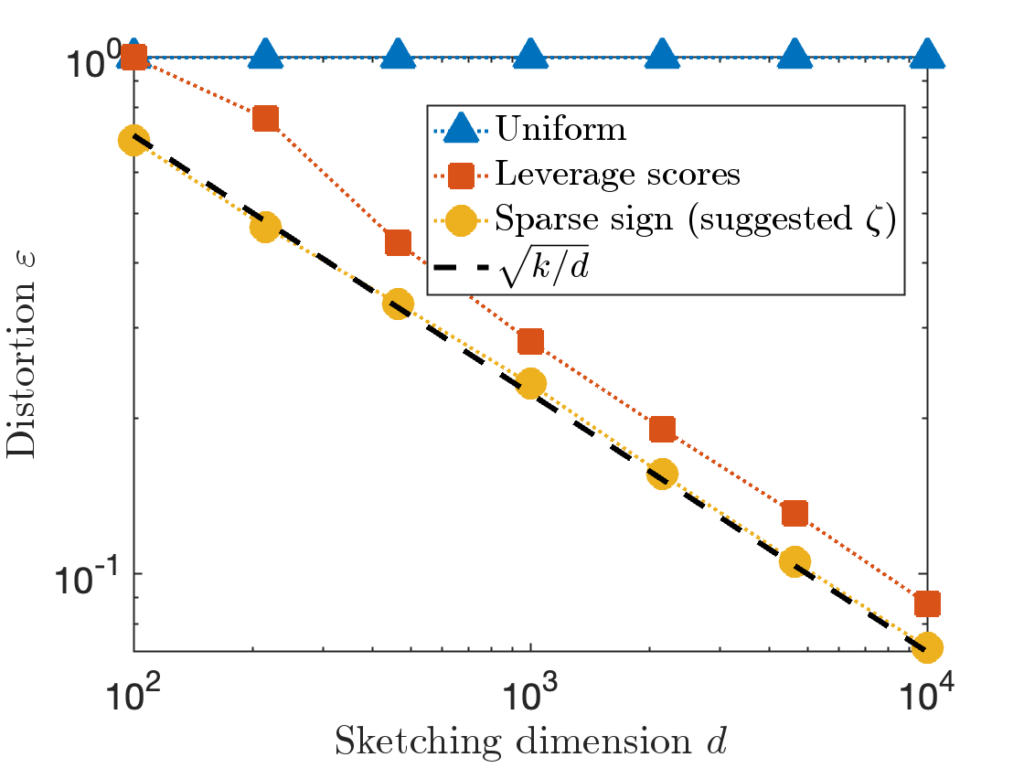
We see right away that the uniform sampling fails dramatically on this problem. That’s to be expected. All but 50 of 100,000 rows of $A$ are zero, so picking rows uniformly at random will give nonsense with very high probability. Uniform sampling can work well for matrices $A$ which are “incoherent”, with all rows of $A$ being of “similar importance”.

Conclusion (Uniform sampling). Uniform sampling is a risky method; it works excellently for some problems, but fails spectacularly for others. Use only with caution!

The ridge leverage score sampling method is more interesting. Unlike all the other sketches we’ve discussed in this post, ridge leverage score sampling is data-dependent. First, it computes a leverage score $\ell_i$ for each row of $A$ and then samples rows with probabilities proportional to these scores. For high enough values of $d$ , ridge leverage score sampling performs slightly (but only slightly) worse than the characteristic $\varepsilon = \sqrt{k/d}$ scaling we expect for an oblivious subspace embedding.

Ultimately, leverage score sampling has two disadvantages when compared with oblivious sketching matrices:

Higher distortion, higher variance. The distortion of a leverage score sketch is higher on average, and more variable, than an oblivious sketch, which achieve very consistent performance.
Computing the leverage scores. In order to implement this sketch, the leverage scores $\ell_i$ have to first be computed or estimated. This is a nontrivial algorithmic problem; the most direct way of computing the leverage scores requires a QR decomposition at $\mathcal{O}(nk^2)$ cost, much higher than other types of sketches.

There are settings when coordinate sampling methods, such as leverage scores, are well-justified:

Structured matrices. For some matrices $A$ , the leverage scores might be very cheap to compute or approximate. In such cases, coordinate sampling can be faster than oblivious sketching.
“Active learning”. For some problems, each entry of the vector $b$ or row of the matrix $A$ may be expensive to generate. In this case, coordinate sampling has the distinct advantage that computing $Sb$ or $SA$ only requires generating the entries of $b$ or rows of $A$ for the $d$ randomly selected indices $i_1,\ldots,i_d$ .

Ultimately, oblivious sketching and coordinate sampling both have their place as tools in the computational toolkit. For the reasons described above, I believe that oblivious sketching should usually be preferred to coordinate sampling in the absence of a special reason to prefer the latter.

Tensor Random Embeddings

There are a number of sketching matrices with tensor structure; see here for a survey. These types of sketching matrices are very well-suited to tensor computations. If tensor structure is present in your application, I would put these types of sketches at the top of my list for consideration.

CountSketch

The CountSketch sketching matrix is the $\zeta = 1$ case of the sparse sign embedding. CountSketch has serious deficiencies, and should only be used in practice with extreme care.

Consider the “Identity” test matrix from above but with parameter $k = 200$ , and compare the distortion of CountSketch to the sparse sign embedding with parameters $\zeta=2,4,8$ :

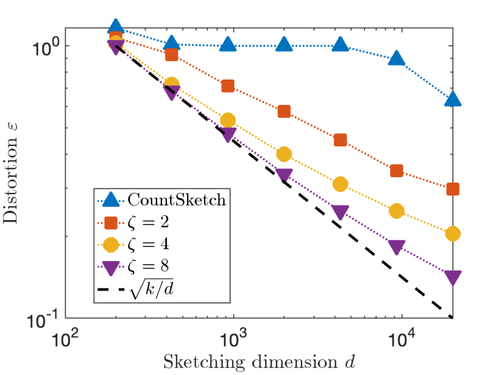
We see that the distortion of the CountSketch remains persistently high at 100% until the sketching dimension $d$ is taken $>4300$ , 20× higher than $k$ .

CountSketch is bad because it requires $d$ to be proportional to $k^2/\varepsilon^2$ in order to achieve distortion $\varepsilon$ . For all of the other sketching matrices we’ve considered, we’ve only required $d$ to be proportional to $k/\varepsilon^2$ (or perhaps $(k\log k)/\varepsilon^2$ ). This difference between $d\propto k^2$ for CountSketch and $d\propto k$ for other sketching matrices is a at the root of CountSketch’s woefully bad performance on some inputs.³

The fact that CountSketch requires $d\propto k^2$ is simple to show. It’s basically a variant on the famous birthday problem. We include a discussion at the end of this post.⁴

There are ways of fixing the CountSketch. For instance, we can use a composite sketch $S = S_2 \cdot S_1$ , where $S_1$ is a CountSketch of size $k^2/\varepsilon^2 \times n$ and $S_2$ is a Gaussian sketching matrix of size $k/\varepsilon^2 \times k^2/\varepsilon^2$ .⁵ For most applications, however, salvaging CountSketch doesn’t seem worth it; sparse sign embeddings with even $\zeta = 2$ nonzeros per column are already way more effective and reliable than a plain CountSketch.

Conclusion

By now, sketching is quite a big field, with dozens of different proposed constructions for sketching matrices. So which should you use? For most use cases, sparse sign embeddings are a good choice; they are fast to construct and apply and offer uniformly good distortion across a range of matrices.

Bonus: CountSketch and the Birthday Problem

The point of this bonus section is to prove the following (informal) theorem:

Let $A$ be the “Identity” test matrix above. If $S\in\real^{d\times n}$ is a CountSketch matrix with output dimension $d\ll k^2$ , then the distortion of $S$ for $\operatorname{col}(A)$ is $\varepsilon\ge 1$ with high probability.

Let’s see why. By the structure of the matrix $A$ , $SA$ has the form

$SA = \begin{bmatrix} s_1 & \cdots & s_k \end{bmatrix}$

where each vector $s_i\in\real^d$ has a single $\pm1$ in a uniformly random location $j\_i$ .

Suppose that the indices $j_1,\ldots,j_k$ are not all different from each other, say $j_i = j_{i'}$ . Set $x = e_i - e_{i'}$ , where $e_i$ is the standard basis vector with $1$ in position $i$ and zeros elsewhere. Then, $(SA)x = 0$ but $\norm{x} = \sqrt{2}$ . Thus, for the distortion relation

$(1-\varepsilon) \norm{x} =(1-\varepsilon)\sqrt{2} \le 0 = \norm{(SA)x}$

to hold, $\varepsilon \ge 1$ . Thus,

$\prob \{ \varepsilon \ge 1 \} \ge \prob \{ j_1,\ldots,j_k \text{ are not distinct} \}.$

For a moment, let’s put aside our analysis of the CountSketch, and turn our attention to a famous puzzle, known as the birthday problem:

How many people have to be in a room before there’s at least a 50% chance that two people share the same birthday?

The counterintuitive or “paradoxical” answer: 23. This is much smaller than many people’s intuition, as there are 365 possible birthdays and 23 is much smaller than 365.

The reason for this surprising result is that, in a room of 23 people, there are ${23 \choose 2} = 23\cdot 22/2=253$ pairs of people. Each pair of people has a $1/365$ chance of sharing a birthday, so the expected number of birthdays in a room of 23 people is $253/365 \approx 0.69$ . Since are 0.69 birthdays shared on average in a room of 23 people, it is perhaps less surprising that 23 is the critical number at which the chance of two people sharing a birthday exceeds 50%.

Hopefully, the similarity between the birthday problem and CountSketch is becoming clear. Each pair of indices $j_i$ and $j_{i'}$ in CountSketch have a $1/d$ chance of being the same. There are ${k\choose 2} \approx k^2/2$ pairs of indices, so the expected number of equal indices $j_i = j_{i'}$ is $\approx k^2/2d$ . Thus, we should anticipate $d \gtrapprox k^2$ is required to ensure that $j_1,\ldots,j_k$ are distinct with high probability.

Let’s calculate things out a bit more precisely. First, realize that

$\prob \{ j_1,\ldots,j_k \text{ are not distinct} \} = 1 - \prob \{ j_1,\ldots,j_k \text{ are distinct} \}.$

To compute the probability that $j_1,\ldots,j_k$ are distinct, imagine introducing each $j_i$ one at a time. Assuming that $j_1,\ldots,j_{i-1}$ are all distinct, the probability $j_1,\ldots,j_i$ are distinct is just the probability that $j_i$ does not take any of the $i-1$ values $j_1,\ldots,j_i$ . This probability is

$\prob\{ j_1,\ldots,j_i \text{ are distinct} \mid j_1,\ldots,j_{i-1} \text{ are distinct}\} = 1 - \frac{i-1}{d}.$

Thus, by the chain rule for probability,

$\prob \{ j_1,\ldots,j_k \text{ are distinct} \} = \prod_{i=1}^k \left(1 - \frac{i-1}{d} \right).$

To bound this quantity, use the numeric inequality $1-x\le \exp(-x)$ for every $x \in \real$ , obtaining

$\mathbb{P} \{ j_1,\ldots,j_k \text{ are distinct} \} \le \prod_{i=0}^{k-1} \exp\left(-\frac{i}{d}\right) = \exp \left( -\frac{1}{d}\sum_{i=0}^{k-1} i \right) = \exp\left(-\frac{k(k-1)}{2d}\right).$

Thus, we conclude that

$\prob \{ \varepsilon \ge 1 \} \ge 1-\prob \{ j_1,\ldots,j_k \text{ are distinct} \\}\ge 1-\exp\left(-\frac{k(k-1)}{2d}\right).$

Solving this inequality, we conclude that

$\prob\{\varepsilon \ge 1\} \ge \frac{1}{2} \quad \text{if} \quad d \le \frac{k(k-1)}{2\ln 2}.$

This is a quantitative version of our informal theorem from earlier.

Experiments

Timing

Distortion

Conclusion

Sparse Sign Embeddings: Theory and Practice

Parameter Choices

Implementation

Other Sketching Matrices

Coordinate Sampling

Tensor Random Embeddings

CountSketch

Conclusion

Leave a Reply Cancel reply