Sparse matrices are an indispensable tool for anyone in computational science. I expect there are a very large number of simulation programs written in scientific research across the country which could be faster by ten to a hundred fold at least just by using sparse matrices! In this post, we’ll give a brief overview what a sparse matrix is and how we can use them to solve problems fast.
A matrix is sparse if most of its entries are zero. There is no precise threshold for what “most” means; Kolda suggests that a matrix have at least 90% of its entries be zero for it to be considered sparse. The number of nonzero entries in a sparse matrix  is denoted by
  . A matrix that is not sparse is said to be dense.
Sparse matrices are truly everywhere. They occur in finite difference, finite element, and finite volume discretizations of partial differential equations. They occur in power systems. They occur in signal processing. They occur in social networks. They occur in intermediate stages in computations with dense rank-structured matrices. They occur in data analysis (along with their higher-order tensor cousins).
Why are sparse matrices so common? In a word, locality. If the  th entry
  of a matrix is nonzero, then this means that row
  and column
  are related in some way to each other according to the the matrix . In many situations, a “thing” is only related to a handful of other “things”; in heat diffusion, for example, the temperature at a point may only depend on the temperatures of nearby points. Thus, if such a locality assumption holds, every row will only have a small number of nonzero entries and the matrix overall will be sparse.
Storing and Multiplying Sparse Matrices
A sparse matrix can be stored efficiently by only storing its nonzero entries, along with the row and column in which these entries occur. By doing this, a sparse matrix can be stored in  space rather than the standard
  for an
  matrix .1Here,
  refers to big-O notation. For the efficiency of many algorithms, it will be very beneficial to store the entries row-by-row or column-by-column using compressed sparse row and column (CSR and CSC) formats; most established scientific programming software environments support sparse matrices stored in one or both of these formats. For efficiency, it is best to enumerate all of the nonzero entries for the entire sparse matrix and then form the sparse matrix using a compressed format all at once. Adding additional entries one at a time to a sparse matrix in a compressed format requires reshuffling the entire data structure for each new nonzero entry.
There exist straightforward algorithms to multiply a sparse matrix stored in a compressed format with a vector  to compute the product
  . Initialize the vector
  to zero and iterate over the nonzero entries of , each time adding
  to
to  . It is easy to see this algorithm runs in time.2More precisely, this algorithm takes
  time since it requires
  operations to initialize the vector even if has no nonzero entries. We shall ignore this subtlety in the remainder of this article and assume that
  , which is true of most sparse matrices occurring in practice The fact that sparse matrix-vector products can be computed quickly makes so-called Krylov subspace iterative methods popular for solving linear algebraic problems involving sparse matrices, as these techniques only interact with the matrix by computing matrix-vector products
  (or matrix-tranpose-vector products
  ).
).
Lest the reader think that every operation with a sparse matrix is necessarily fast, the product of two sparse matrices and  need not be sparse and the time complexity need not be
  . A counterexample is
(1) 
for  . We have that
  but
but
(2) 
which has  nonzero elements and requires operations to compute. However, if one does the multiplication in the other order, one has
  and the multiplication can be done in operations. Thus, some sparse matrices can be multiplied fast and others can’t. This phenomena of different speeds for different sparse matrices is very much also true for solving sparse linear systems of equations.
Solving Sparse Linear Systems
The question of how to solve a sparse system of linear equations  where is sparse is a very deep problems with fascinating connections to graph theory. For this article, we shall concern ourselves with so-called sparse direct methods, which solve by means of computing a factorization of the sparse matrix . These methods produce an exact solution to the system if all computations are performed exactly and are generally considered more robust than inexact and iterative methods. As we shall see, there are fundamental limits on the speed of certain sparse direct methods, which make iterative methods very appealing for some problems.
Note from the outset that our presentation will be on illustrating the big ideas rather than presenting the careful step-by-step details needed to actually code a sparse direct method yourself. An excellent reference for the latter is Tim Davis’ wonderful book Direct Methods for Sparse Linear Systems.
Let us begin by reviewing how  factorization works for general matrices. Suppose that the
  entry of is nonzero. Then, factorization proceeds by subtracting scaled multiples of the first row from the other rows to zero out the first column. If one keeps track of these scaling, then one can write this process as a matrix factorization, which we may demonstrate pictorially as
(3) 
Here,  ‘s denote nonzero entries and blanks denote zero entries. We then repeat the process on the
  submatrix in the bottom right (the so-called Schur complement). Continuing in this way, we eventually end up with a complete factorization
(4) 
In the case that is symmetric positive definite (SPD), one has that  for
for  a diagonal matrix consisting of the entries on
  . This factorization
  is a Cholesky factorization of .3Often, the Cholesky factorization is written as
  for
for  or
or  for
for  . These different forms all contain the same basic information, so we shall stick with the
  formulation in this post. For general non-SPD matrices, one needs to incorporate partial pivoting for Gaussian elimination to produce accurate results.4See the excellent monograph Accuracy and Stability of Numerical Algorithms for a comprehensive treatment of this topic.
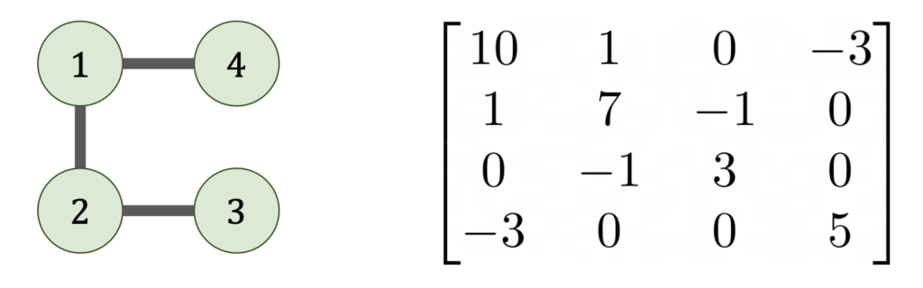
Let’s try the same procedure for a sparse matrix. Consider a sparse matrix with the following sparsity pattern:
(5) 
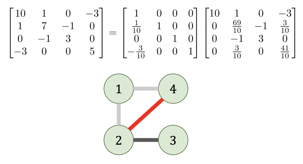
When we eliminate the entry, we get the following factorization:
(6) 
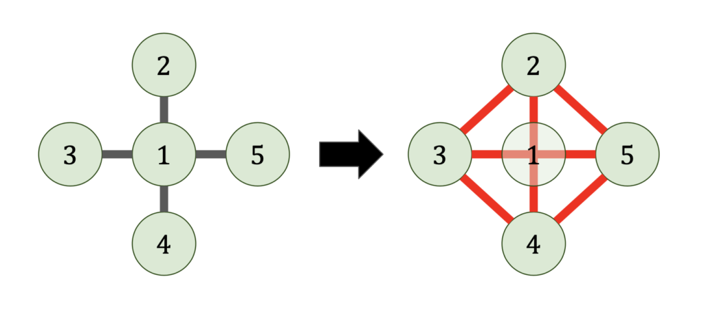
Note that the Schur complement has new additional nonzero entries (marked with a  ) not in the original sparse matrix . The Schur complement of is denser than was; there are new fill-in entries. The worst-case scenario for fill-in is the arrowhead matrix:
(7) 
After one step of Gaussian elimination, we went from a matrix with nonzeros to a fully dense Schur complement! However, the arrowhead matrix also demonstrates a promising strategy. Simply construct a permutation matrix which reorders the first entry to be the last5For instance, the circular shift permutation  . and then perform Gaussian elimination on the symmetrically permuted matrix
  instead. In fact, the entire factorization can be computed without fill-in:
(8) 
This example shows the tremendous importance of reordering of the rows and columns when computing a sparse factorization.
The Best Reordering
As mentioned above, when computing an factorization of a dense matrix, one generally has to reorder the rows (and/or columns) of the matrix to compute the solution accurately. Thus, when computing the factorization of a sparse matrix, one has to balance the need to reorder for accuracy and to reorder to reduce fill-in. For these reasons, for the remainder of this post, we shall focus on computing Cholesky factorizations of SPD sparse matrices, where reordering for accuracy is not necessary.6For ill-conditioned and positive semi-definite matrices, one may want to reorder a Cholesky factorization so the result is rank-revealing. This review article has a good discussion of pivoted Cholesky factorization. For most applications, one can successfully compute an accurate Cholesky factorization without any specific accuracy-focused reordering strategy. Since we want the matrix to remain SPD, we must restrict ourselves to symmetric reordering strategies where is reordered to where  is a permutation matrix.
Our question is deceptively simple: what reordering produces the least fill-in? In matrix language, what permutation minimizes  where
where  is the Cholesky factorization of ?
Note that, assuming no entries in the Gaussian elimination process exactly cancel, then the Cholesky factorization depends only on the sparsity pattern of (the locations of the zeros and nonzeros) and not on the actual numeric values of ‘s entries. This sparsity structure is naturally represented by a graph  whose nodes are the indices
  with an edge between
  if, and only if,
  .
.
Now let’s see what happens when we do Gaussian elimination from a graph point-of-view. When we eliminate the entry from matrix, this results in all nodes of the graph adjacent to  becoming connected to each other.7Graph theoretically, we add a clique containing the nodes adjacent to
This shows why the arrowhead example is so bad. By eliminating the a vertex connected to every node in the graph, the eliminated graph becomes a complete graph.
Reordering the matrix corresponds to choosing in what order the vertices of the graph are eliminated. Choosing the elimination order is then a puzzle game; eliminate all the vertices of the graph in the order that produces the fewest fill-in edges (shown red).8This “graph game” formulation of sparse Gaussian elimination is based on how I learned it from John Gilbert. His slides are an excellent resource for all things sparse matrices!
Finding the best elimination ordering for a sparse matrix (graph) is a good news/bad news situation. For the good news, many graphs possess a perfect elimination ordering, in which no fill-in is produced at all. There is a simple algorithm to determine whether a graph (sparse matrix) possesses a perfect elimination ordering and if so, what it is.9The algorithm is basically just a breadth-first search. Some important classes of graphs can be eliminated perfectly (for instance, trees). More generally, the class of all graphs which can be eliminated perfectly is precisely the set of chordal graphs, which are well-studied in graph theory.
Now for the bad news. The problem of finding the best elimination ordering (with the least fill-in) for a graph is NP-Hard. This means, assuming the widely conjectured result that  , that finding the best elimination ordering would be a hard computational problem than the worst-case
  complexity for doing Gaussian elimination in any ordering! One should not be too pessimistic about this result, however, since (assuming ) all it says is that there exists no polynomial time algorithm guaranteed to produce the absolutely best possible elimination ordering when presented with any graph (sparse matrix). If one is willing to give up on any one of the bolded statements, further progress may be possible. For instance, there exists several good heuristics, which find reasonably good elimination orderings for graphs (sparse matrices) in linear (or nearly linear) time.
Can Sparse Matrices be Eliminated in Linear Time?
Let us think about the best reordering question in a different way. So far, we have asked the question “Can we find the best ordering for a sparse matrix?” But another question is equally important: “How efficiently can we solve a sparse matrix, even with the best possible ordering?”
One might optimistically hope that every sparse matrix possesses an elimination ordering such that its Cholesky factorization can be computed in linear time (in the number of nonzeros), meaning that the amount of time needed to solve is proportional to the amount of data needed to store the sparse matrix .
When one tests a proposition like this, one should consider the extreme cases. If the matrix is dense, then it requires operations to do Gaussian elimination,10This is neglecting the possibility of acceleration by Strassen–type fast matrix multiplication algorithms. For simplicity, we shall ignore these fast multiplication techniques for the remainder of this post and assume dense can be solved no faster than operations. but only has  nonzero entries. Thus, our proposition cannot hold in unmodified form.
An even more concerning counterexample is given by a matrix whose graph is a  2D grid graph.
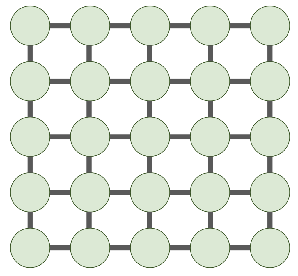
Sparse matrices with this sparsity pattern (or related ones) appear all the time in discretized partial differential equations in two dimensions. Moreover, they are truly sparse, only having  nonzero entries. Unforunately, no linear time elimination ordering exists. We have the following theorem:
Theorem: For any elimination ordering for a sparse matrix with being a  2D grid graph, in any elimination ordering, the Cholesky factorization
  requires
  operations and satisfies
  .11Big-Omega notation is a cousin of Big-O notation. One should read
  as “
as “ is no less than a constant multiple of
  , asymptotically”.
The proof is contained in Theorem 10 and 11 (and the ensuing paragraph) of classic paper by Lipton, Rose, and Tarjan. Natural generalizations to  -dimensional grid graphs give bounds of
  time and
  for
for  . In particular, for 2D finite difference and finite element discretizations, sparse Cholesky factorization takes operations and produces a Cholesky factor with in the best possible ordering. In 3D, sparse Cholesky factorization takes
  operations and produces a Cholesky factor with
  in the best possible ordering.
Fortunately, at least these complexity bounds are attainable: there is an ordering which produces a sparse Cholesky factorization with requiring  operations and with
  nonzero entries in the Cholesky factor.12Big-Theta notation just means
  if
if  and One such asymptotically optimal ordering is the nested dissection ordering, one of the heuristics alluded to in the previous section. The nested dissection ordering proceeds as follows:
- Find a separator
 consisting of a small number of vertices in the graph such that when is removed from , is broken into a small number of edge-disjoint and roughly evenly sized pieces
  .13In particular, is the disjoint union
  and there are no edges between
  and
and  for
for  .
. - Recursively use nested dissection to eliminate each component
 individually.
 - Eliminate in any order.
For example, for the 2D grid graph, if we choose to be a cross through the center of the 2D grid graph, we have a separator of size  dividing the graph into
  roughly
  pieces.
Let us give a brief analysis of this nested dissection ordering. First, consider the sparsity of the Cholesky factor . Let  denote the number of nonzeros in
  for an elimination of the 2D grid graph using the nested dissection ordering. Then step 2 of nested dissection requires us to recursively eliminate four
  2D grid graphs. After doing this, for step 3, all of the vertices of the separator might be connected to each other, so the separator graph will potentially have as many as
  edges, which result in nonzero entries in . Thus, combining the fill-in from both steps, we get
(9) 
Solving this recurrence using the master theorem for recurrences gives  . If one instead wants the time
  required to compute the Cholesky factorization, note that for step 3, in the worst case, all of the vertices of the separator might be connected to each other, leading to a dense matrix. Since a matrix requires
  , we get the recurrence
(10) 
which solves to  .
.
Conclusions
As we’ve seen, sparse direct methods (as exemplified here by sparse Cholesky) possess fundamental scalability challenges for solving large problems. For the important class of 2D and 3D discretized partial differential equations, the time to solve scales like and  , respectively. For truly large-scale problems, these limitations may be prohibitive for using such methods.
This really is the beginning of the story, not the end for sparse matrices however. The scalability challenges for classical sparse direct methods has spawned many exciting different approaches, each of which combats the scalability challenges of sparse direct methods for a different class of sparse matrices in a different way.
Upshot: Sparse matrices occur everywhere in applied mathematics, and many operations on them can be done very fast. However, the speed of computing an factorization of a sparse matrix depends significantly on the arrangement of its nonzero entries. Many sparse matrices can be factored quickly, but some require significant time to factor in any reordering.
5 thoughts on “Big Ideas in Applied Math: Sparse Matrices”