In this post, I want to discuss a very beautiful piece of mathematics I stumbled upon recently. As a warning, this post will be more mathematical than most, but I will still try and sand off the roughest mathematical edges. This post is adapted from a much more comprehensive post by Paata Ivanishvili. My goal is to distill the main idea to its essence, deferring the stochastic calculus until it cannot be avoided.
Jensen’s inequality is one of the most important results in probability.
Jensen’s inequality. Let
be a (real) random variable and
a convex function such that both
and
are defined. Then
.
Here is the standard proof. A convex function has supporting lines. That is, at a point  , there exists a slope
  such that
  for all
  . Invoke this result at
  and
and  and take expectations to conclude that
![\[\mathbb{E}[m(X - \mathbb{E}X) + f(\mathbb{E}X)] = f(\mathbb{E}X) \le \mathbb{E} [f(X)].\]](https://www.ethanepperly.com/wp-content/ql-cache/quicklatex.com-c162fcb6103e44c65d3c6e1d003135d0_l3.png "Rendered by QuickLaTeX.com")
In this post, I will outline a proof of Jensen’s inequality which is much longer and more complicated. Why do this? This more difficult proof illustrates an incredible powerful technique for proving inequalities, interpolation. The interpolation method can be used to prove a number of difficult and useful inequalities in probability theory and beyond. As an example, at the end of this post, we will see the Gaussian Jensen inequality, a striking generalization of Jensen’s inequality with many applications.
The idea of interpolation is as follows: Suppose I wish to prove  for two numbers
  and
and  . This may hard to do directly. With the interpolation method, I first construct a family of numbers
  ,
,  , such that
  and
and  and show that
  is (weakly) increasing in
  . This is typically accomplished by showing the derivative is nonnegative:
![\[\frac{d}{dt} A_t \ge 0.\]](https://www.ethanepperly.com/wp-content/ql-cache/quicklatex.com-7d87bd05d1a5b326f575b2b72f27cc74_l3.png "Rendered by QuickLaTeX.com")
To prove Jensen’s inequality by interpolation, we shall begin with a special case. As often in probability, the simplest case is that of a Gaussian random variable.
Jensen’s inequality for a Gaussian. Let
) and let
for some
for any Gaussian random variable
. Then
![\[f(0) \le \mathbb{E} [f(X)].\]](https://www.ethanepperly.com/wp-content/ql-cache/quicklatex.com-8e5dd3a04978ca82dd4d50fd41f8ca43_l3.png "Rendered by QuickLaTeX.com")
Note that the conclusion is exactly Jensen’s inequality, as we have assumed is mean-zero.
The difficulty with any proof by interpolation is to come up with the “right” . For us, the “right” answer will take the form
![\[A_t = \mathbb{E} [ f(X_t) ],\]](https://www.ethanepperly.com/wp-content/ql-cache/quicklatex.com-8f12251961aff234ee138a29978a264b_l3.png "Rendered by QuickLaTeX.com")
where  starts with no randomness and
  is our standard Gaussian. To interpolate between these extremes, we increase the variance linearly from
  to . Thus, we define
![\[A_t = \mathbb{E} [ f(X_t)] \quad \text{where $X_t\sim\mathcal{N}(0,t)$}.\]](https://www.ethanepperly.com/wp-content/ql-cache/quicklatex.com-88cc0a1a3f5c52e8349fd6c4ca28ad7c_l3.png "Rendered by QuickLaTeX.com")
Here, and throughout,  denotes a Gaussian random variable with zero mean and variance
  .
.
Let’s compute the derivative of . To do this, let  denote a small parameter which we will later send to zero. For us, the key fact will be that a
  can be realized as a sum of independent
  and
and  random variables. Therefore, we write
![\[X_{t+\delta} = X_t + \Delta \quad \text{where $\Delta \sim \mathcal{N}(0,\delta)$ is independent of $X_t$.}\]](https://www.ethanepperly.com/wp-content/ql-cache/quicklatex.com-eaaa1bd888269b9ad51b88afb5fc3d08_l3.png "Rendered by QuickLaTeX.com")
We now evaluate  by using Taylor’s formula
(1) ![\[f(X_t+\Delta) = f(X_t) + f'(X_t)\Delta + \frac{1}{2} f''(X_t) \Delta^2 + \frac{1}{6} f'''(\xi) \Delta^3, \]](https://www.ethanepperly.com/wp-content/ql-cache/quicklatex.com-38d38dde93cc24a3101649064d5af389_l3.png "Rendered by QuickLaTeX.com")
where  lies between
  and
and  . Now, take expectations,
![\[\mathbb{E}[ f(X_t+\Delta)]=\mathbb{E}[f(X_t)] + \mathbb{E}[f'(X_t)\Delta] + \frac{1}{2} \mathbb{E}[f''(X_t)] \mathbb{E}[\Delta^2] + \underbrace{\frac{1}{6} \mathbb{E}[f'''(\xi) \Delta^3]}_{:=\mathrm{Rem}(\delta)}.\]](https://www.ethanepperly.com/wp-content/ql-cache/quicklatex.com-ccacfa2622a31446e66624a9a8458dc4_l3.png "Rendered by QuickLaTeX.com")
The random variable  has mean zero and variance
  so this gives
![\[\mathbb{E} [f(X_t+\Delta)]=\mathbb{E}[f(X_t)] + \delta \frac{1}{2} \mathbb{E}[f''(X_t)] + \mathrm{Rem}(\delta).\]](https://www.ethanepperly.com/wp-content/ql-cache/quicklatex.com-d021f960b2367c41cf18dc25661045c6_l3.png "Rendered by QuickLaTeX.com")
As we show below, the remainder term  vanishes as
  . Thus, we can rearrange this expression to compute the derivative:
![\[\frac{d}{dt} A_t = \lim_{\delta \downarrow 0} \frac{\mathbb{E} f(X_t+\Delta)-\mathbb{E}[f(X_t)]}{\delta} = \lim_{\delta \downarrow 0} \frac{1}{2} \mathbb{E}[f''(X_t)] + \frac{\mathrm{Rem}(\delta)}{\delta} = \frac{1}{2} \mathbb{E}[f''(X_t)].\]](https://www.ethanepperly.com/wp-content/ql-cache/quicklatex.com-3275fd914e25d0f6985eb4d1ca419fb7_l3.png "Rendered by QuickLaTeX.com")
The second derivative of a convex function is nonnegative:  for every
  . Therefore,
![\[\frac{d}{dt} A_t \ge 0 \quad \text{for all } t\in [0,1].\]](https://www.ethanepperly.com/wp-content/ql-cache/quicklatex.com-258c784d449d2b53c0a462ff38f3cdd8_l3.png "Rendered by QuickLaTeX.com")
Jensen’s inequality is proven! In fact, we’ve proven the stronger version of Jensen’s inequality:
![\[\mathbb{E} f(X) = f(0) + \frac{1}{2} \int_0^1 \mathbb{E} [f''(X_t)] \, dt.\]](https://www.ethanepperly.com/wp-content/ql-cache/quicklatex.com-50be5d67c30ff436025f45185c2fae22_l3.png "Rendered by QuickLaTeX.com")
This strengthened version can yield improvements. For instance, if  is
is  -smooth
![\[f''(x) \le \beta \quad \text{for every } x \in \real,\]](https://www.ethanepperly.com/wp-content/ql-cache/quicklatex.com-206d02bd0b654ab4c42cf33921d5383d_l3.png "Rendered by QuickLaTeX.com")
then we have
![\[f(0) \le \mathbb{E} f(X) \le f(0) + \frac{1}{2}\beta.\]](https://www.ethanepperly.com/wp-content/ql-cache/quicklatex.com-8561680db386f740b927a84c7cb9fe0d_l3.png "Rendered by QuickLaTeX.com")
This inequality isn’t too hard to prove directly, but it does show that we’ve obtained something more than the simple proof of Jensen’s inequality.
as  . Let’s do this. As an exercise, you can verify that our technical regularity condition implies
  . Thus, by Hölder’s inequality and setting
  to be
to be  ‘s Hölder conjugate (
 ), we obtain
 ![\[\frac{|\mathrm{Rem}(\delta)|}{\delta} = \frac{|\mathbb{E}[f'''(\xi) \Delta^3]|}{6\delta} \le \frac{(|\mathbb{E} |f'''(\xi)|^p)^{1/p}| (\mathbb{E} |\Delta|^{3q})^{1/q}}{6\delta}.\]](https://www.ethanepperly.com/wp-content/ql-cache/quicklatex.com-e1078e0f2d2c17b77bd87a38665c03e4_l3.png "Rendered by QuickLaTeX.com")
One can show that
 where
where  is a function of alone. Therefore,
  as
as  .
.What’s Really Going On Here?
In our proof, we use a family of random variables  , defined for each
  . Rather than treating these quantities as independent, we can think of them as a collective, comprising a random function
  known as a Brownian motion.
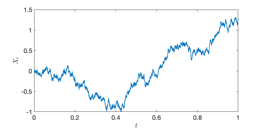
The Brownian motion is a very natural way of interpolating between a constant  and a Gaussian with mean .2The Ornstein–Uhlenbeck process is another natural way of interpolating between a random variable and a Gaussian.
There is an entire subject known as stochastic calculus which allows us to perform computations with Brownian motion and other random processes. The rules of stochastic calculus can seem bizarre at first. For a function of a real number , we often write
![\[df = f'(x) \, dx\]](https://www.ethanepperly.com/wp-content/ql-cache/quicklatex.com-a32870f7f5981a412b96de2591534280_l3.png "Rendered by QuickLaTeX.com")
For a function  of a Brownian motion, the analog is Itô’s formula
![\[df = f'(X_t) \, dX_t + \frac{1}{2} f''(X_t) \, dt.\]](https://www.ethanepperly.com/wp-content/ql-cache/quicklatex.com-e2eadd9f0624f41b562d90fe0568ef69_l3.png "Rendered by QuickLaTeX.com")
While this might seem odd at first, this formula may seem more sensible if we compare with (1) above. The idea, very roughly, is that for an increment of the Brownian motion  over a time interval
  ,
,  is a random variable with mean , so we cannot drop the second term in the Taylor series, even up to first order in . Fully diving into the subtleties of stochastic calculus is far beyond the scope of this short post. Hopefully, the rest of this post, which outlines some extensions of our proof of Jensen’s inequality that require more stochastic calculus, will serve as an enticement to learn more about this beautiful subject.
Proving Jensen by Interpolation
For the rest of this post, we will be less careful with mathematical technicalities. We can use the same idea that we used to prove Jensen’s inequality for a Gaussian random variable to prove Jensen’s inequality for any random variable  :
:
![\[f(\mathbb{E}Y) \le \mathbb{E}[f(Y)].\]](https://www.ethanepperly.com/wp-content/ql-cache/quicklatex.com-97693077e012820448760d2e7ad31d58_l3.png "Rendered by QuickLaTeX.com")
Here is the idea of the proof.
First, realize that we can write any random variable as a function of a standard Gaussian random variable . Indeed, letting  and
and  denote the cumulative distribution functions of and , one can show that
![\[g(X) := \inf \{ \alpha \in \real : F_Y(\alpha) \ge F_X(X) \}\]](https://www.ethanepperly.com/wp-content/ql-cache/quicklatex.com-2c40cdc3f3bcf589f930aeb87340491b_l3.png "Rendered by QuickLaTeX.com")
has the same distribution as .
Now, as before, we can interpolate between  and using a Brownian motion. As a first, idea, we might try
![\[A_t \stackrel{?}{=} \mathbb{E} [f(g(X_t))].\]](https://www.ethanepperly.com/wp-content/ql-cache/quicklatex.com-0de3d1811026212f153ea79469649149_l3.png "Rendered by QuickLaTeX.com")
Unfortunately, this choice of does not work! Indeed, ![A_0 = \mathbb{E}[f(g(0))]](https://www.ethanepperly.com/wp-content/ql-cache/quicklatex.com-e6ac6421e3fc94f2087614f41336491a_l3.png "Rendered by QuickLaTeX.com") does not even equal to
does not even equal to ![\mathbb{E} [f(Y)]](https://www.ethanepperly.com/wp-content/ql-cache/quicklatex.com-06983640d9e119e9aa44cdd209c540c7_l3.png "Rendered by QuickLaTeX.com") ! Instead, we must define
! Instead, we must define
![\[A_t = \mathbb{E} [f(\mathbb{E}[g(X_1) \mid X_t])].\]](https://www.ethanepperly.com/wp-content/ql-cache/quicklatex.com-19560c3c89aa3987101e6650af24a0a7_l3.png "Rendered by QuickLaTeX.com")
We define using the conditional expectation of the final value  conditional on the Brownian motion at an earlier time . Using a bit of elbow grease and stochastic calculus, one can show that
![\[\frac{d}{dt} A_t \ge 0 \quad \text{for all }t\in [0,1].\]](https://www.ethanepperly.com/wp-content/ql-cache/quicklatex.com-253003b644ae67d253cdfd74378c71a9_l3.png "Rendered by QuickLaTeX.com")
This provides a proof of Jensen’s inequality in general by the method if interpolation.
Gaussian Jensen Inequality
Now, we’ve come to the real treat, the Gaussian Jensen inequality. In the last section, we saw the sketch of a proof of Jensen’s inequality using interpolation. While it is cool that this proof is possible, we learned anything new since we can prove Jensen’s inequality in other ways. The Gaussian Jensen inequality provides an application of this technique which is hard to prove other ways. This section, in particular, is cribbing quite heavily from Paata Ivanishvili‘s excellent post on the topic.
Here’s the big question:
If
are “somewhat dependent”, for which functions does the multivariate Jensen’s inequality
(
hold?)
![\[f(\mathbb{E} Y_1,\ldots,\mathbb{E}Y_n) \le \mathbb{E} [f(Y_1,\ldots,Y_n)] \]](https://www.ethanepperly.com/wp-content/ql-cache/quicklatex.com-2467fe840ba04173b1a3adc7c38a945c_l3.png "Rendered by QuickLaTeX.com")
Considering extreme cases, if are entirely dependent, then we would only expect () to hold when is convex. But if are independent, then we can apply Jensen’s inequality to each coordinate one at a time to deduce
![\[\text{($\star$) holds if $f$ is convex in each coordinate, separately.}\]](https://www.ethanepperly.com/wp-content/ql-cache/quicklatex.com-521f389e0e1a83728c2544ecb889a047_l3.png "Rendered by QuickLaTeX.com")
We would like a result which interpolates between extremes {fully dependent, fully convex} and {independent, separately convex}. The Gaussian Jensen inequality provides exactly this tool.
As in the previous section, we can generate arbitrary random variables as functions  of Gaussian random variables
  . We will use the covariance matrix
  of the Gaussian random variables as our measure of the dependence of the random variables . With this preparation in place, we have the following result:
Gaussian Jensen inequality. The conclusion of Jensen’s inequality
(2)
holds for all test functionsif and only if
Here,
is the Hessian matrix at
denotes the entrywise product of matrices.
![\[f(\mathbb{E}g_1(X_1),\ldots,\mathbb{E}g_n(X_n)) \le \mathbb{E} [f(g(X_1),\ldots,g(X_n))]\]](https://www.ethanepperly.com/wp-content/ql-cache/quicklatex.com-055c60480c4de2b28348bb1da12763ea_l3.png "Rendered by QuickLaTeX.com")
![\[\Sigma \circ \nabla^2 f(x) \text{ is positive semidefinite} \quad \text{for all $x \in \real^n$}.\]](https://www.ethanepperly.com/wp-content/ql-cache/quicklatex.com-48ca7d18e3bbcee337d072bd27efe791_l3.png "Rendered by QuickLaTeX.com")
This is a beautiful result with striking consequences (see Ivanishvili‘s post). The proof is essentially the same as the proof as Jensen’s inequality by interpolation with a little additional bookkeeping.
Let us confirm this result respects our extreme cases. In the case where  are equal (and variance one), is a matrix of all ones and
  for all . Thus, the Gaussian Jensen inequality states that (2) holds if and only if is positive semidefinite for every , which occurs precisely when is convex.
Next, suppose that are independent and variance one, then is the identity matrix and
![\[\Sigma \circ \nabla^2 f(x) = \mathrm{diag} \left( \frac{\partial^2 f}{\partial x_i^2} : i=1,\ldots,n \right).\]](https://www.ethanepperly.com/wp-content/ql-cache/quicklatex.com-ef80f7d5a452131378d194e3560717b0_l3.png "Rendered by QuickLaTeX.com")
A diagonal matrix is positive semidefinite if and only if its entries are nonnegative. Thus, (2) holds if and only if each of ‘s diagonal second derivatives are nonnegative  : this is precisely the condition for to be separately convex in each argument.
There’s much more to be said about the Gaussian Jensen inequality, and I encourage you to read Ivanishvili‘s post to see the proof and applications. What I find so compelling about this result—so compelling that I felt the need to write this post—is how interpolation and stochastic calculus can be used to prove inequalities which don’t feel like stochastic calculus problems. The Gaussian Jensen inequality is a statement about functions of dependent Gaussian random variables; there’s nothing dynamic happening. Yet, to prove this result, we inject dynamics into the problem, viewing the two sides of our inequality as endpoints of a random process connecting them. This is a such a beautiful idea that I couldn’t help but share it.
 . At each step, the user makes one of two choices:
 .
. , if the state is
  , the probability of moving to state
  is a fixed number
  . In particular, the probability
  by
by  . Note that the states
 ![\[\mathbb{P} \{ x_{n+1} = j \mid x_n = i,x_{n-1}=a_{n-1},\ldots,x_0=a_0\} = \mathbb{P}\{x_{n+1} = j \mid x_n = i\} = P_{ij}.\]](https://www.ethanepperly.com/wp-content/ql-cache/quicklatex.com-d1fa5c29673402a40f530434ec99f998_l3.png "Rendered by QuickLaTeX.com")
 given the entire history of the system depends only on the value
  of the chain at time
  .
. ). Thus,
  )
) ![\[P_{ij} = \frac{0.15}{m}. \]](https://www.ethanepperly.com/wp-content/ql-cache/quicklatex.com-e9cb5a0e824c976c19d2d73c1f45714b_l3.png "Rendered by QuickLaTeX.com")
 outgoing links. Then, in addition to the
  probability computed before, user
  chance of picking
  )
) ![\[P_{ij} = \frac{0.85}{d_i} + \frac{0.15}{m}. \]](https://www.ethanepperly.com/wp-content/ql-cache/quicklatex.com-51a6f3c00da58822f6465db8458a1f8c_l3.png "Rendered by QuickLaTeX.com")
 , we can understand the processes evolution by determining its state
  at every point in time
  of the process at every time
  by a row vector
  .
. is a column vector but
  stores the probability that the system is in state
  for every
  ).
). denote the probability distributions of the states
  . It is natural to ask: How are the distributions
  is in state
  :
:![\[\rho^{(n+1)}_j = \mathbb{P} \{x_{n+1} = j\}\]](https://www.ethanepperly.com/wp-content/ql-cache/quicklatex.com-d8705a90b65f869a58cd432bbc884cfa_l3.png "Rendered by QuickLaTeX.com")
 or
or  or … or
  ; only one of these cases can be true at once. When we have an “or” of random events and these events are
 ![\[\rho^{(n+1)}_j = \mathbb{P} \{x_{n+1} = j\} = \sum_{i=1}^m \mathbb{P} \{x_{n+1} = j, x_n = i\}.\]](https://www.ethanepperly.com/wp-content/ql-cache/quicklatex.com-448c23761c566dc3504d60b57f1ac8d1_l3.png "Rendered by QuickLaTeX.com")
 and
and ![\[\rho^{(n+1)}_j = \sum_{i=1}^m \mathbb{P} \{x_{n+1} = j, x_n = i\} = \sum_{i=1}^m \mathbb{P} \{x_n = i\} \mathbb{P}\{x_{n+1} = j \mid x_n = i\}.\]](https://www.ethanepperly.com/wp-content/ql-cache/quicklatex.com-9b27f4d81b8b51c36f578f7e00017d96_l3.png "Rendered by QuickLaTeX.com")
 and the probability of moving from
 ![\[\rho_j^{(n+1)} = \sum_{i=1}^m \rho^{(n)}_i P_{ij} .\]](https://www.ethanepperly.com/wp-content/ql-cache/quicklatex.com-1a858376daf68ec5f2d816ef52e66997_l3.png "Rendered by QuickLaTeX.com")
![\[\left(\rho^{(n+1)}\right)^\top = \left(\rho^{(n)}\right)^\top P \quad \text{for any } n = 0,1,2,\ldots.\]](https://www.ethanepperly.com/wp-content/ql-cache/quicklatex.com-9ae710d7c26dc66ed497cc8faf34cab3_l3.png "Rendered by QuickLaTeX.com")
 matrix
  , then the distribution at time
 ![\[\left(\rho^{(n)}\right)^\top = \left(\rho^{(n-1)}\right)^\top P = \left[\left(\rho^{(n-2)}\right)^\top P\right]P = \left(\rho^{(n-2)}\right)^\top P^2 = \cdots = \left(\rho^{(0)}\right)^\top P^n.\]](https://www.ethanepperly.com/wp-content/ql-cache/quicklatex.com-3fddd821b8cdb4b89262b0c72ea68e55_l3.png "Rendered by QuickLaTeX.com")
 at time
  converge to a single fixed probability distribution
  regardless of how the chain is initialized (i.e., independent of the starting distribution
 ![\[\pi^\top = \pi^\top P. \]](https://www.ethanepperly.com/wp-content/ql-cache/quicklatex.com-daa1101ffcda26584d5f843c12765158_l3.png "Rendered by QuickLaTeX.com")
![\[\left(\rho^{(n+1)}\right)^\top = \left(\rho^{(n)}\right)^\top P,\]](https://www.ethanepperly.com/wp-content/ql-cache/quicklatex.com-bcbc3e101491a613c1dcb40680a4ef3b_l3.png "Rendered by QuickLaTeX.com")
 , and observe that both
  and
and  converge to
  .
.![\[\text{There exists $n$ such that, for any $i,j = 1,2,\ldots,m$, } \quad\mathbb{P}\{x_n = j \mid x_0 = i \} = (P^n)_{ij} > 0.\]](https://www.ethanepperly.com/wp-content/ql-cache/quicklatex.com-9796d227fdde3830779ea16f255b9b70_l3.png "Rendered by QuickLaTeX.com")
 converge to
  step, there is at least a
  chance of moving from any website
  and you’re interested in where your traffic is coming from. One way of achieving this would be to initialize the Markov chain at
  as our initial distribution for
  is defined as follows: The probability
  of moving from
 ![\[\mathbb{P} \{y_1 = j \mid y_0 = i\} = P^{\rm rev}_{ij} = \mathbb{P} \{ x_0 = j \mid x_1 = i \}.\]](https://www.ethanepperly.com/wp-content/ql-cache/quicklatex.com-caeb5343a623f571314596e612b7315d_l3.png "Rendered by QuickLaTeX.com")
![\[P^{\rm rev}_{ij} = \mathbb{P} \{ x_0 = j \mid x_1 = i \} = \frac{\mathbb{P} \{x_0 = j\} \mathbb{P} \{x_1 = i \mid x_0 = j\}}{\mathbb{P} \{x_1 = i\}} = \frac{ \pi_j P_{ji}}{\pi_i}. \]](https://www.ethanepperly.com/wp-content/ql-cache/quicklatex.com-1ffaf13a6eb4a6d8079f1ee0f7501d5d_l3.png "Rendered by QuickLaTeX.com")
 at their website and following the chain one step back.
![\[P^{\rm rev}_{ij} = P_{ij} \quad \text{for every } i,j=1,2,\ldots,m.\]](https://www.ethanepperly.com/wp-content/ql-cache/quicklatex.com-4d394cf7f8d6b8a6318c27c3e447403d_l3.png "Rendered by QuickLaTeX.com")
![\[\pi_i P_{ij} = \pi_j P_{ji}.\]](https://www.ethanepperly.com/wp-content/ql-cache/quicklatex.com-d6dade4e26238f165b12b7d2891d3a95_l3.png "Rendered by QuickLaTeX.com")
 as defining a function on the set
  ,
,  . Letting
  , we can define a non-standard
  :
: ![\langle f, g\rangle_{\pi} \coloneqq \mathbb{E}[f(x) g(x)] = \sum_{i=1}^m \pi_i f(i)g(i)](https://www.ethanepperly.com/wp-content/ql-cache/quicklatex.com-1c871929113a513c08da0e9fa24a8043_l3.png "Rendered by QuickLaTeX.com") . Then the Markov chain is reversible if and only if detailed balance holds if and only if
. Then the Markov chain is reversible if and only if detailed balance holds if and only if  . This more abstract characterization has useful consequences. For instance, by the
  ) is equal to the flow of probability mass from
  ).
). :
:![\[\sigma_i P_{ij} = \sigma_j P_{ji}.\]](https://www.ethanepperly.com/wp-content/ql-cache/quicklatex.com-f1ef7062af77b1ad2efc526c3db8a63b_l3.png "Rendered by QuickLaTeX.com")
 is the stationary distribution of this chain. To see why, we check the stationarity condition
  . Indeed, for every
 ![\[(\sigma^\top P)_j = \sum_{i=1}^m \sigma_i P_{ij} = \sum_{i=1}^m \sigma_j P_{ji} = \sigma_j.\]](https://www.ethanepperly.com/wp-content/ql-cache/quicklatex.com-81a7b02ba8de821bb56ecee978ec346d_l3.png "Rendered by QuickLaTeX.com")
 such that
  for every
  . The proposal distribution
  add to one:
  .
. , then
  .
.![\[\min \left\{ 1 , \frac{\pi_j T_{ji}}{\pi_i T_{ij}} \right\}.\]](https://www.ethanepperly.com/wp-content/ql-cache/quicklatex.com-fb8ef7791b1d955015f1300e0eddfb8c_l3.png "Rendered by QuickLaTeX.com")
 . This Markov chain is known as a
  .
. with from the proposal distribution,
  .
.![\[p_{\rm acc} := \min \left\{ 1 , \frac{\pi_j T_{ji}}{\pi_i T_{ij}} \right\}.\]](https://www.ethanepperly.com/wp-content/ql-cache/quicklatex.com-e34abfe410068f7516cd1c5e50100c3c_l3.png "Rendered by QuickLaTeX.com")
 , set
, set  . Otherwise, set
  .
. and go back to step 2.
 under the Metropolis–Hastings sampler is the proposal probability
 ![\[P_{ij} = T_{ij} \cdot \min \left\{ 1 , \frac{\pi_j T_{ji}}{\pi_i T_{ij}} \right\}.\]](https://www.ethanepperly.com/wp-content/ql-cache/quicklatex.com-8c98e72078f3de5c0de43a1683f5d406_l3.png "Rendered by QuickLaTeX.com")
 is always satisfied for any Markov chain
  .
.![\[\pi_i P_{ij} = \pi_i T_{ij} \cdot \min \left\{ 1 , \frac{\pi_j T_{ji}}{\pi_i T_{ij}} \right\} = \min \left\{ \pi_i T_{ij} , \pi_j T_{ji} \right\} = \pi_j P_{ji}.\]](https://www.ethanepperly.com/wp-content/ql-cache/quicklatex.com-9ec53c4f48f0cc7bb8cc1d0cd58750f1_l3.png "Rendered by QuickLaTeX.com")
 different baked goods. I want to pick out
  special items for a display window to lure customers into my store. As a first approach, I might pick my top-
 for my baked goods. In the
  th entry
  of my matrix, I write the number of sales for baked good
  of my matrix with a measure of similarity between items
  be the number ordered for each bakery item by a random customer. Set
  being the correlation between the random variables
  and
and  . The matrix
  be a diagonal matrix where
  is the total sales of item
  . By scaling
  of picking items
  is proportional to the
  . More specifically,
![\[\pi_S = \frac{\det A(S,S)}{\sum_{\text{all subsets $T$ of size $k$}} \det A(T,T)}. \]](https://www.ethanepperly.com/wp-content/ql-cache/quicklatex.com-26714c8980fc33f439de8cf1e5a692eb_l3.png "Rendered by QuickLaTeX.com")
 submatrix of
  . Such a random subset is known as a
  items and a display case of size
  . Suppose I have three items: a pumpkin muffin, a chocolate chip muffin, and an oatmeal raisin cookies. Say the
 ![\[A = \begin{bmatrix} 10 & 9 & 0 \\ 9 & 10 & 0 \\ 0 & 0 & 5 \end{bmatrix}.\]](https://www.ethanepperly.com/wp-content/ql-cache/quicklatex.com-b8bb20f6bff68d835397eabaf8a1cdc0_l3.png "Rendered by QuickLaTeX.com")
 and much more popular than the cookie
  . However, the two muffins are similar to each other and thus the corresponding submatrix has small determinant
![\[\det A(\{1,2\},\{1,2\}) = \det \twobytwo{10}{9}{9}{10} = 19.\]](https://www.ethanepperly.com/wp-content/ql-cache/quicklatex.com-7f74f9426bb0c808b9e4384a0a2a6c2d_l3.png "Rendered by QuickLaTeX.com")
![\[\det A(\{1,3\},\{1,3\}) = \det A(\{2,3\},\{2,3\}) = \det \twobytwo{10}{0}{0}{5} = 50.\]](https://www.ethanepperly.com/wp-content/ql-cache/quicklatex.com-812d8318cba1d4a937e92858658ff7e8_l3.png "Rendered by QuickLaTeX.com")
 -DPP, we have a
  chance of choosing a muffin and a cookie for our display case. It is for this reason that we can say that a
  possible
  items and want to pick
  of them, there are already over 10 trillion possible combinations.
 . To generate a proposal, choose a uniformly random element
  out of
  and a uniformly random element
  out of
  without
  obtained from
  ).
).![\[p_{\rm acc} = \min \left\{ 1 , \frac{\pi_{S'} T_{S'S}}{\pi_{S} T_{SS'}} \right\}.\]](https://www.ethanepperly.com/wp-content/ql-cache/quicklatex.com-5ff5280a20cfddd08b7917152edbfb68_l3.png "Rendered by QuickLaTeX.com")
 and
and  are both equal to
  ,
,  . Using the formula for the probability
 ![\[\frac{\pi_{S'}}{\pi_S} = \frac{\det A(S',S')}{\det A(S,S)}.\]](https://www.ethanepperly.com/wp-content/ql-cache/quicklatex.com-26f4fdbc4d7624e49904e22703e8aaa7_l3.png "Rendered by QuickLaTeX.com")
![\[p_{\rm acc} = \min \left\{ 1 , \frac{\pi_{S'} T_{S'S}}{\pi_{S} T_{SS'}} \right\} = \min \left\{ 1, \frac{\det A(S',S')}{\det A(S,S)} \right\}. \]](https://www.ethanepperly.com/wp-content/ql-cache/quicklatex.com-16c835576499e7fb3e6cf2c219732873_l3.png "Rendered by QuickLaTeX.com")
 arbitrarily and set
  .
. .
. .
. . Otherwise, set
  .
. steps.
 entries of the matrix
  be a standard Gaussian vector—that is, a vector populated by independent
  of
of  denotes the
 ![\[\|g\| = \sqrt{g_1^2 + \cdots + g_n^2},\]](https://www.ethanepperly.com/wp-content/ql-cache/quicklatex.com-284e0c747adfdfc57c90b3d282798075_l3.png "Rendered by QuickLaTeX.com")


![\[\mathbb{E} \|g\| = \sqrt{2} \frac{\Gamma((n+1)/2)}{\Gamma(n/2)},\]](https://www.ethanepperly.com/wp-content/ql-cache/quicklatex.com-274737e67b7cf65854623497d2336e99_l3.png "Rendered by QuickLaTeX.com")
 is the
 ![\[\sqrt{n-1} < \frac{n}{\sqrt{n+1}} < \mathbb{E} \|g\| < \sqrt{n}. \]](https://www.ethanepperly.com/wp-content/ql-cache/quicklatex.com-074224f9e909d1c2a33cfadb8b37e771_l3.png "Rendered by QuickLaTeX.com")
 . The authors of
  and
and  , we have
![\[\frac{x}{(x+s)^{1-s}} < \frac{\Gamma(x+s)}{\Gamma(x)} < x^s. \]](https://www.ethanepperly.com/wp-content/ql-cache/quicklatex.com-52ca1feab59cc018c9d7af7cbf54afd7_l3.png "Rendered by QuickLaTeX.com")
 and
and  and multiply by
  to obtain
![\[\frac{\sqrt{2} \cdot n/2}{(n/2+1/2)^{1/2}} < \sqrt{2}\frac{\Gamma((n+1)/2)}{\Gamma(n/2)} = \mathbb{E}\|g\| < \sqrt{2}\cdot \sqrt{n/2},\]](https://www.ethanepperly.com/wp-content/ql-cache/quicklatex.com-9bbede5bad09ae09b80d77db4e728b62_l3.png "Rendered by QuickLaTeX.com")
 and
and ![\[\Gamma((1-s)x + sy) < \Gamma(x)^{1-s} \Gamma(y)^s. \]](https://www.ethanepperly.com/wp-content/ql-cache/quicklatex.com-53b31e91194bbc5f8b440c65b868feb4_l3.png "Rendered by QuickLaTeX.com")
 to obtain
![\[\Gamma(x+s) = \Gamma((1-s)x + s(x+1)) < \Gamma(x)^{1-s} \Gamma(x+1)^s.\]](https://www.ethanepperly.com/wp-content/ql-cache/quicklatex.com-00f0550f27637fb27d0ab53fb8892bff_l3.png "Rendered by QuickLaTeX.com")
 and use
  to conclude
![\[\frac{\Gamma(x+s)}{\Gamma(x)} < \left( \frac{\Gamma(x+1)}{\Gamma(x)} \right)^s = x^s. \]](https://www.ethanepperly.com/wp-content/ql-cache/quicklatex.com-3607c86e6e40b082b75960abc24dca1c_l3.png "Rendered by QuickLaTeX.com")
 in place of
  in place of
  to obtain
![\[\frac{\Gamma(x+1)}{\Gamma(x+s)} < (x+s)^{1-s}.\]](https://www.ethanepperly.com/wp-content/ql-cache/quicklatex.com-6c2671296814cc9b8138d5143fc9d6a9_l3.png "Rendered by QuickLaTeX.com")
 , dividing by
  , and using
 ![\[\frac{\Gamma(x+s)}{\Gamma(x)} > \frac{\Gamma(x+1)}{\Gamma(x)} \cdot \frac{1}{(x+s)^{1-s}} = \frac{x}{(x+s)^{1-s}},\]](https://www.ethanepperly.com/wp-content/ql-cache/quicklatex.com-0d742ab239498d1540847646ffabaa9c_l3.png "Rendered by QuickLaTeX.com")
 , where we use the fact that
  is the sum of
  follows from a weaker version of Wendel’s inequality,
  ,
,![\[\Var(f(g)) \le \mathbb{E} \| \nabla f(g)\|^2.\]](https://www.ethanepperly.com/wp-content/ql-cache/quicklatex.com-456ec9d3ca714d36d760fccd6f3a452c_l3.png "Rendered by QuickLaTeX.com")
 which has gradient
  . Thus,
![\[\mathbb{E} \| \nabla f(g)\|^2 = 1 \ge \Var(f(g)) = \mathbb{E} \|g\|^2 - (\mathbb{E} \|g\|)^2 = n - (\mathbb{E} \|g\|)^2.\]](https://www.ethanepperly.com/wp-content/ql-cache/quicklatex.com-b806bd5311f18368939fef93576bf328_l3.png "Rendered by QuickLaTeX.com")
 , estimate its trace
  .
.![\[\hat{\tr} = \frac{1}{m} \sum_{i=1}^m \omega_i^* A \omega_i. \]](https://www.ethanepperly.com/wp-content/ql-cache/quicklatex.com-a287886ee24c9ab99dfe35b6cdae83cf_l3.png "Rendered by QuickLaTeX.com")
 are random vectors, usually chosen to be
  denotes the
  .
.![\[\mathbb{E} [\omega_i\omega_i^*] = I, \]](https://www.ethanepperly.com/wp-content/ql-cache/quicklatex.com-74bb76367ad1408bd538d049774cf990_l3.png "Rendered by QuickLaTeX.com")
![\[\mathbb{E} [\hat{\tr}] = \tr A.\]](https://www.ethanepperly.com/wp-content/ql-cache/quicklatex.com-f6407c7a741003cc20780e72d050cb56_l3.png "Rendered by QuickLaTeX.com")
![\[\mathbb{E} [\hat{\tr}] = \mathbb{E} \left[ \frac{1}{m} \sum_{i=1}^m \omega_i^*A\omega_i \right] = \frac{1}{m} \sum_{i=1}^m \mathbb{E} \left[ \omega_i^* A \omega_i\right]. \]](https://www.ethanepperly.com/wp-content/ql-cache/quicklatex.com-52eebd003a597cac5b2c69f7b6e537e8_l3.png "Rendered by QuickLaTeX.com")
![\mathbb{E} [\hat{\tr}] = \tr A](https://www.ethanepperly.com/wp-content/ql-cache/quicklatex.com-96f71a1b054ffed9e316cf9cb7a16c5c_l3.png "Rendered by QuickLaTeX.com") , it is sufficient to prove that
, it is sufficient to prove that ![\mathbb{E} \left[\omega_i^*A\omega_i\right] = \tr A](https://www.ethanepperly.com/wp-content/ql-cache/quicklatex.com-120169dca277175c51f09b6f320cf5fa_l3.png "Rendered by QuickLaTeX.com") for each
for each  matrix, then a number equals its trace,
  . The second trick is the
  matrix
  and a
and a  matrix
  , we have
  . The cyclic property
 ![\[\tr[BCD] = \tr[(BC)D] = \tr[D(BC)] = \tr[DBC].\]](https://www.ethanepperly.com/wp-content/ql-cache/quicklatex.com-cc1cd4920a2431e93b5453b5373999e3_l3.png "Rendered by QuickLaTeX.com")
![\[\tr [BCD] \ne \tr[CBD] \quad \text{in general}.\]](https://www.ethanepperly.com/wp-content/ql-cache/quicklatex.com-f563660fc58383a37ae7bedea16b2b9c_l3.png "Rendered by QuickLaTeX.com")
 as beads on a closed loop of string. One can move the last bead
 ![\tr [BCD] = \tr[DBC]](https://www.ethanepperly.com/wp-content/ql-cache/quicklatex.com-7656627b133add21ab8765532def07d6_l3.png "Rendered by QuickLaTeX.com") , but not interchange two beads,
, but not interchange two beads, ![\tr[BCD] \ne \tr[CBD]](https://www.ethanepperly.com/wp-content/ql-cache/quicklatex.com-0f43e4f72510a69b596f7b9f7504dd58_l3.png "Rendered by QuickLaTeX.com") .
.![\[\mathbb{E} \left[\omega_i^*A\omega_i\right] = \mathbb{E} \tr \left[\omega_i^*A\omega_i\right] = \mathbb{E} \tr \left[A\omega_i\omega_i^*\right].\]](https://www.ethanepperly.com/wp-content/ql-cache/quicklatex.com-b1bb373766e64179bc0635f058a07f3f_l3.png "Rendered by QuickLaTeX.com")
![\[\mathbb{E} \left[\omega_i^*A\omega_i\right] = \mathbb{E} \tr \left[A\omega_i\omega_i^*\right] = \tr(A \mathbb{E}[\omega_i\omega_i^*] ).\]](https://www.ethanepperly.com/wp-content/ql-cache/quicklatex.com-1d10f835c99efab005f0ad12cdb5647b_l3.png "Rendered by QuickLaTeX.com")
![\[\mathbb{E} \left[\omega_i^*A\omega_i\right] = \tr(A \mathbb{E}[\omega_i\omega_i^*] ) = \tr(A\cdot I) = \tr A.\]](https://www.ethanepperly.com/wp-content/ql-cache/quicklatex.com-b51781498146df3547c1503e451ad682_l3.png "Rendered by QuickLaTeX.com")
 ‘s are isotropic (3) and now assume that
 ![\[\Var(\hat{\tr}) = \frac{1}{m^2} \sum_{i=1}^m \Var(\omega_i^*A\omega_i).\]](https://www.ethanepperly.com/wp-content/ql-cache/quicklatex.com-d9398dc43178ba9bb72aead0214e77c8_l3.png "Rendered by QuickLaTeX.com")
 , we then get
![\[\Var(\hat{\tr}) = \frac{1}{m} \Var(\omega^*A\omega).\]](https://www.ethanepperly.com/wp-content/ql-cache/quicklatex.com-4501a18842234362f8f99d523c7c723e_l3.png "Rendered by QuickLaTeX.com")
 is unbiased (i.e, (3)), this means that the mean square error decays like
 ![\[\left| \hat{\tr} - \tr A \right| \lessapprox \frac{\mathrm{const}}{\sqrt{m}}.\]](https://www.ethanepperly.com/wp-content/ql-cache/quicklatex.com-c735791b8fe88d627bc2ebad8137fb1e_l3.png "Rendered by QuickLaTeX.com")
 , I must do
  the work!
 and (root-mean-square) error at rates
 ![\[\Var(\hat{\tr}_{\text{H++ or X}}) \le \frac{\mathrm{const}}{m^2},\quad \left| \hat{\tr}_{\text{H++ or X}} - \tr A \right| \lessapprox \frac{\mathrm{const}}{m}.\]](https://www.ethanepperly.com/wp-content/ql-cache/quicklatex.com-87438d87094d3df389400b5f7abee24a_l3.png "Rendered by QuickLaTeX.com")
 that makes the variance of the single–sample estimate
  as low as possible. In this section, we will provide several explicit formulas for the variance of the Girard–Hutchinson estimator. Derivations of these formulas will appear at the end of this post. These variance formulas help illuminate the benefits and drawbacks of different test vector distributions.
 we use
  and
and  to denote the real and imaginary parts. The variance of a random complex number
  is
is![\[\Var(z) := \mathbb{E} |z - \mathbb{E} z|^2 = \Var(\Re z) + \Var(\Im z).\]](https://www.ethanepperly.com/wp-content/ql-cache/quicklatex.com-8f636667a7dbbb3217896a962de1d28c_l3.png "Rendered by QuickLaTeX.com")
![\[\left\|A\right\|_{\rm F}^2 = \sum_{i,j} |A_{ij}|^2.\]](https://www.ethanepperly.com/wp-content/ql-cache/quicklatex.com-e132e4b9029c41dbfb99cd0e588d8d70_l3.png "Rendered by QuickLaTeX.com")
 , we have
![\[\left\|A\right\|_{\rm F}^2 = \sum_{i=1}^n \lambda_i^2. \]](https://www.ethanepperly.com/wp-content/ql-cache/quicklatex.com-06b272e602552353c020f6399347c748_l3.png "Rendered by QuickLaTeX.com")
 denotes the
  denotes the
  rather than the conjugate transpose
  is a number, it is equal to its own transpose:
![\[\omega^\top A \omega = (\omega^\top A \omega)^\top = \omega^\top A^\top \omega.\]](https://www.ethanepperly.com/wp-content/ql-cache/quicklatex.com-3d543dc0d4d64d3c28f0f291cd9c8e83_l3.png "Rendered by QuickLaTeX.com")
![\[\omega^\top A\omega = \frac{\omega^\top A \omega + \omega^\top A^\top \omega}{2} = \omega^\top \left( \frac{A + A^\top}{2} \right)\omega.\]](https://www.ethanepperly.com/wp-content/ql-cache/quicklatex.com-f1bbe4f0c983f73e2461b593b752f54a_l3.png "Rendered by QuickLaTeX.com")
 .
. .
.![\[\Var(\omega^\top A\omega) = 2 \left\|A\right\|_{\rm F}^2.\]](https://www.ethanepperly.com/wp-content/ql-cache/quicklatex.com-091cf638fab943be5fd224acdb42668f_l3.png "Rendered by QuickLaTeX.com")

![\[\Var(\omega^\top A \omega) = 2\sum_{i\ne j} |A_{ij}|^2.\]](https://www.ethanepperly.com/wp-content/ql-cache/quicklatex.com-74621dad79cb3f06a8b70c661df4e01d_l3.png "Rendered by QuickLaTeX.com")
 are uniformly distributed on the real sphere of radius
  .
. ![\[\Var(\omega^\top A\omega) = \frac{2n}{n+2} \left( \left\|A\right\|_{\rm F}^2 - \frac{1}{n} |\tr A|^2 \right).\]](https://www.ethanepperly.com/wp-content/ql-cache/quicklatex.com-1e419b8da9b953a0b8b914df9e89f8c6_l3.png "Rendered by QuickLaTeX.com")
![\[A = A^{\rm H} + i A^{\rm SH}\]](https://www.ethanepperly.com/wp-content/ql-cache/quicklatex.com-d61da43cd6497ceefd2306aabb52ee67_l3.png "Rendered by QuickLaTeX.com")
![\[A^{\rm H} = \frac{A+A^*}{2} ,\quad A^{\rm SH} = \frac{A - A^*}{2i}\]](https://www.ethanepperly.com/wp-content/ql-cache/quicklatex.com-dc287a49a59dca9421fdd2bef6be5334_l3.png "Rendered by QuickLaTeX.com")
 is skew-Hermitian). Since
  and
and  are both Hermitian, we have
![\[\Re(\omega^* A\omega) = \omega^* A^{\rm H} \omega, \quad \Im (\omega^* A \omega) = \omega^* A^{\rm SH} \omega.\]](https://www.ethanepperly.com/wp-content/ql-cache/quicklatex.com-6809a35cd06d92218ce8d597847f74bd_l3.png "Rendered by QuickLaTeX.com")
 can be broken into Hermitian and skew-Hermitian parts:
![\[\Var(\omega^* A\omega) = \Var(\omega^* A^{\rm H}\omega) + \Var(\omega^* A^{\rm SH}\omega).\]](https://www.ethanepperly.com/wp-content/ql-cache/quicklatex.com-e4658c38df479c5805dabd94b64cc0b3_l3.png "Rendered by QuickLaTeX.com")
 .
. for
for  standard normal random variables.
 ![\[\Var(\omega^* A\omega) = \left\|A\right\|_{\rm F}^2.\]](https://www.ethanepperly.com/wp-content/ql-cache/quicklatex.com-1beb66e032d83431dac6f8e0d6655eec_l3.png "Rendered by QuickLaTeX.com")
 .
. ![\[\Var(\omega^* A \omega) = \sum_{i\ne j} |A_{ij}|^2.\]](https://www.ethanepperly.com/wp-content/ql-cache/quicklatex.com-1cb0e8df66c34056cd350752070af17a_l3.png "Rendered by QuickLaTeX.com")
 .
. ![\[\Var(\omega^* A\omega) = \frac{n}{n+1} \left( \left\|A\right\|_{\rm F}^2 - \frac{1}{n} |\tr A|^2 \right).\]](https://www.ethanepperly.com/wp-content/ql-cache/quicklatex.com-aacfa2afb45905f6abe0697c769cd1b7_l3.png "Rendered by QuickLaTeX.com")
 are isotropic (2), independent from each other, and have independent entries, then for any fixed real symmetric matrix
  .
. -valued and an
  -valued test vectors on unified footing, let
  denote either
  ) or a complex Hermitian matrix (if
  ). Let a
  of
of ![\[\text{If $A \in \mathscr{A}$ and $U$ is $\field$-unitary, then $U^*AU \in \mathscr{A}$.}\]](https://www.ethanepperly.com/wp-content/ql-cache/quicklatex.com-18b4216d44b2364ea39ed4a078a067af_l3.png "Rendered by QuickLaTeX.com")
 is minimized by choosing
  .
. , the set of all
  , where
  is
is  is a diagonal matrix reporting
  has the same distribution as
  . Therefore,
![\[\Var(\omega^\top A \omega) = \Var(\omega^\top \Lambda \omega) = \Var \left( \sum_{i=1}^n \lambda_i \omega_i^2 \right) = \sum_{i=1}^n \lambda_i^2 \Var(\omega_i^2) = 2\sum_{i=1}^n \lambda_i^2 = 2\left\|A\right\|_{\rm F}^2.\]](https://www.ethanepperly.com/wp-content/ql-cache/quicklatex.com-a7416823720bac922fae7cc685892a49_l3.png "Rendered by QuickLaTeX.com")
 . Thus,
![\[\Var(\omega^\top A \omega) = \Var(\omega^\top \mathfrak{R}(A) \omega) + \Var(\omega^\top \mathfrak{I}(A) \omega) = 2\left\|\mathfrak{R}(A)\right\|_{\rm F}^2 + 2\left\|\mathfrak{I}(A)\right\|_{\rm F}^2 = 2\left\|A\right\|_{\rm F}^2.\]](https://www.ethanepperly.com/wp-content/ql-cache/quicklatex.com-527980eb3510f2c015106e6945126d41_l3.png "Rendered by QuickLaTeX.com")
![\[\omega^\top A \omega - \mathbb{E}[\omega^\top A \omega] = \sum_{i,j=1}^n A_{ij} \omega_i\omega_j - \sum_{i=1}^n A_{ii} = \sum_{i\ne j} A_{ij} \omega_i\omega_j + \sum_{i=1}^n A_{ii}(\omega_i^2-1).\]](https://www.ethanepperly.com/wp-content/ql-cache/quicklatex.com-4489cc9cb97ee7a0896bc61193d79910_l3.png "Rendered by QuickLaTeX.com")
 for every
  can be replaced by two times the sum over
  :
:![\[\omega^\top A \omega - \mathbb{E}[\omega^\top A \omega] = 2\sum_{i< j} A_{ij} \omega_i\omega_j.\]](https://www.ethanepperly.com/wp-content/ql-cache/quicklatex.com-afc5f6bb40cd00b7897f25d73751f4ca_l3.png "Rendered by QuickLaTeX.com")
 are
are ![\[\Var(a_1 X_1+\cdots+a_kX_k) = |a_1|^2 \Var(X_1) + \cdots + |a_k|^2 \Var(X_k)\]](https://www.ethanepperly.com/wp-content/ql-cache/quicklatex.com-b6fd81d15f564f514f79ab4c33d133d8_l3.png "Rendered by QuickLaTeX.com")
 and numbers
  . Ergo,
![\begin{align*}\Var(\omega^\top A\omega) &= \Var(\omega^\top A \omega - \mathbb{E}[\omega^\top A \omega]) \\&= \Var\left(\sum_{i< j} 2A_{ij} \omega_i\omega_j\right) \\&= \sum_{i<j} 4 |A_{ij}|^2 \Var(\omega_i\omega_j) \\&= \sum_{i<j} 4 |A_{ij}|^2 \\&= 2 \sum_{i\ne j} |A_{ij}|^2.\end{align*}](https://www.ethanepperly.com/wp-content/ql-cache/quicklatex.com-bbb33f378fabd391c28d938420d3a32b_l3.png "Rendered by QuickLaTeX.com")
 is a uniform random sign, which has variance
  camels, the second son took
  camels, the third son
  camels and the wise man took his own camel and went away.
 is easy. Fortunately, we already know such a distribution, the Gaussian distribution, for which we already calculated
  .
.![\[g = \sqrt{\frac{a}{n}} \omega,\]](https://www.ethanepperly.com/wp-content/ql-cache/quicklatex.com-a93345cf94749f98e715e42bc796501c_l3.png "Rendered by QuickLaTeX.com")
 is the squared length of the Gaussian vector
 using the
 ![\[\Var(g^\top A g) = \mathbb{E}[\Var(g^\top A g \mid a)] + \Var(\mathbb{E}[g^\top A g \mid a]).\]](https://www.ethanepperly.com/wp-content/ql-cache/quicklatex.com-e4e5ed235fbf5b2e026bcc58bd23becc_l3.png "Rendered by QuickLaTeX.com")
 and
and ![\mathbb{E}[ \cdot \mid a]](https://www.ethanepperly.com/wp-content/ql-cache/quicklatex.com-6035d77442675ac2f790cfb5417e1072_l3.png "Rendered by QuickLaTeX.com") denote the
denote the  and treating
 ![\begin{align*}\Var(g^\top A g) &= \mathbb{E}[\Var(a/n \cdot \omega^\top A \omega \mid a)] + \Var(\mathbb{E}[a/n \cdot \omega^\top A \omega \mid a]) \\&=\mathbb{E}[(a/n)^2\Var(\omega^\top A \omega)] + \Var(a/n \cdot \mathbb{E}[\omega^\top A \omega]) \\&= \frac{1}{n^2} \mathbb{E}[a^2] \cdot \Var(\omega^\top A \omega) + \frac{1}{n^2} \Var(a) |\mathbb{E} [\omega^\top A \omega]|^2.\end{align*}](https://www.ethanepperly.com/wp-content/ql-cache/quicklatex.com-be052caddf1d08941925fa0283784635_l3.png "Rendered by QuickLaTeX.com")
![\mathbb{E}[a^2]](https://www.ethanepperly.com/wp-content/ql-cache/quicklatex.com-53042ba72cdd3991b14b5d4508da6564_l3.png "Rendered by QuickLaTeX.com") and
and  are known quantities that
 ![\[\mathbb{E}[a^2] = n(n+2), \quad \Var(a) = 2n.\]](https://www.ethanepperly.com/wp-content/ql-cache/quicklatex.com-59ecda0ea21d92e43e3182d5cc5a7217_l3.png "Rendered by QuickLaTeX.com")
![\mathbb{E} [\omega^\top A \omega] = \tr A](https://www.ethanepperly.com/wp-content/ql-cache/quicklatex.com-293908b9583df45d93349435d76b981a_l3.png "Rendered by QuickLaTeX.com") . Plugging these all in, we get
. Plugging these all in, we get![\[2\left\|A\right\|_{\rm F}^2 = \frac{n+2}{n} \Var(\omega^\top A\omega) + \frac{2}{n} |\tr A|^2.\]](https://www.ethanepperly.com/wp-content/ql-cache/quicklatex.com-1c9b70fd4e5bc6ca4006114830d45619_l3.png "Rendered by QuickLaTeX.com")
![\[\Var(\omega^\top A\omega) = \frac{2n}{n+2} \left( \left\|A\right\|_{\rm F}^2 - \frac{1}{n}|\tr A|^2\right).\]](https://www.ethanepperly.com/wp-content/ql-cache/quicklatex.com-7ab53e5895f9a1f474f5bf99fbec5662_l3.png "Rendered by QuickLaTeX.com")
![\[\Var(\omega^*A \omega) = \Var \left( \sum_{i=1}^n \lambda_i |\omega_i|^2 \right) = \sum_{i=1}^n \Var(|\omega_i|^2) \lambda_i^2 = \sum_{i=1}^n \lambda_i^2 = \left\|A\right\|_{\rm F}^2.\]](https://www.ethanepperly.com/wp-content/ql-cache/quicklatex.com-68f4685a4cd845b98fc1a8fd1494e00a_l3.png "Rendered by QuickLaTeX.com")
 is a
is a  ) reveals that
![\[\Var\left( \omega^* A \omega \right) = \Var \left( \sum_{i<j} 2 \Re(A_{ij} \overline{\omega_i} \omega_j) \right).\]](https://www.ethanepperly.com/wp-content/ql-cache/quicklatex.com-b0e61723c22b056d1aca51694c407e6d_l3.png "Rendered by QuickLaTeX.com")
 are
are ![\[\Var\left( \omega^* A \omega \right) = \Var \left( \sum_{i<j} 2 \Re(A_{ij} \overline{\omega_i} \omega_j) \right) = 4\sum_{i<j} \Var \left( \Re(A_{ij} \overline{\omega_i} \omega_j) \right).\]](https://www.ethanepperly.com/wp-content/ql-cache/quicklatex.com-f2d77eb554a1e1ffbe4370efd8c704fb_l3.png "Rendered by QuickLaTeX.com")
 is uniformly distributed on the complex unit circle, we can assume without loss of generality that
  . Thus, letting
  be uniform on the complex unit circle,
![\[\Var\left( \omega^* A \omega \right) = 4\sum_{i<j} \Var \left( |A_{ij}|\Re(\phi)) \right) = 4\Var\left( \Re(\phi) \right)\sum_{i<j}|A_{ij}|^2.\]](https://www.ethanepperly.com/wp-content/ql-cache/quicklatex.com-76d2ce84714c4549a86686259bd96847_l3.png "Rendered by QuickLaTeX.com")
![\[1 = \Var(\phi) = \Var(\Re \phi) + \Var(\Im \phi) = 2 \Var(\Re \phi)\]](https://www.ethanepperly.com/wp-content/ql-cache/quicklatex.com-f83462ae4de80311482849de445edd5a_l3.png "Rendered by QuickLaTeX.com")
 . Thus
![\[\Var\left( \omega^* A \omega \right) = 2 \sum_{i<j}|A_{ij}|^2 = \sum_{i\ne j} |A_{ij}|^2.\]](https://www.ethanepperly.com/wp-content/ql-cache/quicklatex.com-436eeb79ad0eddde0752f1a398397ad5_l3.png "Rendered by QuickLaTeX.com")
 and
and  denote the real and imaginary parts of a vector or matrix, taken entrywise. The key insight is that if
 ![\[\mathscr{R}(\omega) := \twobyone{\mathfrak{R}(\omega)}{\mathfrak{I}(\omega)}\in\real^{2n} \quad \text{is a uniform random vector on the real sphere of radius $\sqrt{n}$}.\]](https://www.ethanepperly.com/wp-content/ql-cache/quicklatex.com-0ff873eff96e863cf02d36e65a5ca1be_l3.png "Rendered by QuickLaTeX.com")
 .
. . To do this, recall that one way of representing complex numbers is by
  matrices:
![\[a + bi \iff \twobytwo{a}{-b}{b}{a}.\]](https://www.ethanepperly.com/wp-content/ql-cache/quicklatex.com-21b802836b33431568e5d854455d87d1_l3.png "Rendered by QuickLaTeX.com")
![\[\mathscr{R}(A) = \twobytwo{\mathfrak{R}(A)}{-\mathfrak{I}(A)}{\mathfrak{I}(A)}{\mathfrak{R}(A)}.\]](https://www.ethanepperly.com/wp-content/ql-cache/quicklatex.com-12a37c4298c9e2d49dfa2f3ac32fe573_l3.png "Rendered by QuickLaTeX.com")
![\[\mathscr{R}(A + B) = \mathscr{R}(A) + \mathscr{R}(B), \quad \mathscr{R}(A\cdot B) = \mathscr{R}(A) \cdot \mathscr{R}(B)\]](https://www.ethanepperly.com/wp-content/ql-cache/quicklatex.com-4e7fe7da4edb58f1ee1bb8a2b1d2a78b_l3.png "Rendered by QuickLaTeX.com")
 . A short calculation reveals
![\[\omega^*A\omega = \mathscr{R}(\omega)^\top \mathscr{R}(A)\mathscr{R}(\omega) .\]](https://www.ethanepperly.com/wp-content/ql-cache/quicklatex.com-d92927d567b8907621af83ab283672a5_l3.png "Rendered by QuickLaTeX.com")
 is a uniform random vector on the sphere of radius
  . Thus, by the variance formula for the real sphere, we get
![\[\Var(\omega^*A\omega) = \Var[(\sqrt{2}\mathscr{R}(\omega))^\top (\mathscr{R}(A)/2)(\sqrt{2}\mathscr{R}(\omega) )] = \frac{4n}{2n+2} \left[ \|\mathscr{R}(A)/2\|_{\rm F}^2 - \frac{1}{8n}(\tr\mathscr{R}(A))^2 \right].\]](https://www.ethanepperly.com/wp-content/ql-cache/quicklatex.com-ff16ba8dd015218ea642633d77f2a37a_l3.png "Rendered by QuickLaTeX.com")
 and
and  . Plugging this in, we obtain
![\[\Var(\omega^*A\omega)= \frac{n}{n+1} \left[ \|A\|_{\rm F}^2 - \frac{1}{n}(\tr A)^2 \right].\]](https://www.ethanepperly.com/wp-content/ql-cache/quicklatex.com-c9186eb813af3cd67173d73e32885a22_l3.png "Rendered by QuickLaTeX.com")
![\[\mathbb{E} [(\omega^*A \omega)^2].\]](https://www.ethanepperly.com/wp-content/ql-cache/quicklatex.com-8e3e10402f389b06dcd42db97c5ed116_l3.png "Rendered by QuickLaTeX.com")
 . For those unfamiliar with the tensor product, the main properties we will be using
 ![\[(A\otimes B) (C\otimes D) = (AB) \otimes (CD), \quad \tr(A\otimes B) = \tr A \cdot \tr B. \]](https://www.ethanepperly.com/wp-content/ql-cache/quicklatex.com-c5ea1a0235766ad15b67d02b47cfea2e_l3.png "Rendered by QuickLaTeX.com")
![\[\omega^* A \omega = \tr (\omega^*A\omega) = \tr (A \omega\omega^*).\]](https://www.ethanepperly.com/wp-content/ql-cache/quicklatex.com-578bb521ecfb65fc4025f13431673b08_l3.png "Rendered by QuickLaTeX.com")
![\[(\omega^*A\omega)^2 = (\tr [A \omega\omega^*])^2 = \tr [A\omega\omega^* \otimes A\omega\omega^*] = \tr [(A\otimes A) (\omega\omega^* \otimes \omega\omega^*)].\]](https://www.ethanepperly.com/wp-content/ql-cache/quicklatex.com-5161bc0d787be08130c4cfaed0c84489_l3.png "Rendered by QuickLaTeX.com")
![\mathbb{E}[(\omega^*A\omega)^2]](https://www.ethanepperly.com/wp-content/ql-cache/quicklatex.com-98fe9a5e8220c22709c9d6ade6c3141b_l3.png "Rendered by QuickLaTeX.com") , it will be sufficient to evaluate
, it will be sufficient to evaluate ![\mathbb{E}[\omega\omega^* \otimes \omega\omega^*]](https://www.ethanepperly.com/wp-content/ql-cache/quicklatex.com-06ac3d64041068176a86563cec4c67ba_l3.png "Rendered by QuickLaTeX.com") . Forunately, there is a useful formula for these expectation provided by a field of mathematics known as representation theory (see Lemma 1 in
. Forunately, there is a useful formula for these expectation provided by a field of mathematics known as representation theory (see Lemma 1 in ![\[\mathbb{E}[ \omega\omega^* \otimes \omega\omega^*] = \frac{2n}{n+1} \operatorname{Proj}_{\operatorname{Sym}^2(\complex^n)}.\]](https://www.ethanepperly.com/wp-content/ql-cache/quicklatex.com-e5eddca3275c6bbb82fa6b789efe7664_l3.png "Rendered by QuickLaTeX.com")
 is the
  . Therefore, we have that
![\[\mathbb{E}[(\omega^*A\omega)^2] = \tr [(A\otimes A) \mathbb{E}(\omega\omega^* \otimes \omega\omega^*)] = \frac{2n}{n+1} \tr [(A\otimes A) \operatorname{Proj}_{\operatorname{Sym}^2(\complex^n)}].\]](https://www.ethanepperly.com/wp-content/ql-cache/quicklatex.com-6c4f09e537808effd6c51c0aa4d20f6e_l3.png "Rendered by QuickLaTeX.com")
![\[\tr \left[(A\otimes B) \operatorname{Proj}_{\operatorname{Sym}^2(\complex^n)}\right] = \frac{1}{2} \left( \tr(AB) + \tr A \cdot \tr B \right).\]](https://www.ethanepperly.com/wp-content/ql-cache/quicklatex.com-3ea7660d7e72964cf11ef2239731a497_l3.png "Rendered by QuickLaTeX.com")
![\begin{align*}\Var(\omega^* A \omega) &= \mathbb{E}[(\omega^*A\omega)^2] - (\mathbb{E}[\omega^*A\omega])^2 \\&= \frac{2n}{n+1}\tr [(A\otimes A) \operatorname{Proj}_{\operatorname{Sym}^2(\complex^n)}] - (\tr A)^2 \\&= \frac{n}{n+1}\left[ \tr A^2 + (\tr A)^2 \right] - (\tr A)^2 \\&= \frac{n}{n+1}\left[ \left\|A\right\|_{\rm F}^2 - \frac{1}{n} (\tr A)^2 \right].\end{align*}](https://www.ethanepperly.com/wp-content/ql-cache/quicklatex.com-7af313e9e07f20b93b0de83867f20a04_l3.png "Rendered by QuickLaTeX.com")
![\[\mathbb{E}[\omega\omega^\top] = I\]](https://www.ethanepperly.com/wp-content/ql-cache/quicklatex.com-232c1e956304b14a7a6f4b55f9ba35e3_l3.png "Rendered by QuickLaTeX.com")
![\mathbb{E}[\omega_i\omega_j] = \delta_{ij}](https://www.ethanepperly.com/wp-content/ql-cache/quicklatex.com-9986528214c0653217367aca2a90d568_l3.png "Rendered by QuickLaTeX.com") , where
, where ![\begin{align*}\mathbb{E}[ (\omega^*A \omega)^2] &= \mathbb{E}\left[ \left( \sum_{i=1}^n A_{ii} \omega_i^2 +2 \sum_{i<j} A_{ij}\omega_i\omega_j) \right)^2\right] \\&= \sum_{i=1}^n A_{ii}^2 \mathbb{E}[\omega_i^4] + \sum_{i<j} (2A_{ii}A_{jj}+4A_{ij}^2) \mathbb{E}[\omega_i^2]\mathbb{E}[\omega_j^2] \\&= \sum_{i=1}^n A_{ii}^2 \mathbb{E}[\omega_i^4] + \sum_{i<j} (2A_{ii}A_{jj}+4A_{ij}^2) .\end{align*}](https://www.ethanepperly.com/wp-content/ql-cache/quicklatex.com-4115914a6e648438e66028437f38ef2a_l3.png "Rendered by QuickLaTeX.com")
![\[\Var(\omega^*A\omega) = \mathbb{E}[ (\omega^*A \omega)^2] - (\mathbb{E}[\omega^* A \omega])^2 = \sum_{i=1}^n A_{ii}^2 (\mathbb{E}[|\omega_i|^4]-1) + 4\sum_{i<j} A_{ij}^2.\]](https://www.ethanepperly.com/wp-content/ql-cache/quicklatex.com-006e2eb8d5f2162654d8c2de39f5a8bc_l3.png "Rendered by QuickLaTeX.com")
 as small as possible. Since
  , the smallest possible value for
  , which is obtained by populating
 ![\[\omega = a \cdot s \quad \text{for} \quad a \in [0,+\infty), \: s \in\{x\in \field^n : x^*x = n \}.\]](https://www.ethanepperly.com/wp-content/ql-cache/quicklatex.com-11867b7bff40d97d79a74d5136774fd9_l3.png "Rendered by QuickLaTeX.com")
![\[\sup_{A\in\mathscr{A}} \Var(\tilde{\omega}^*A\tilde{\omega}) \le \sup_{A\in\mathscr{A}} \Var(\omega^*A\omega \]](https://www.ethanepperly.com/wp-content/ql-cache/quicklatex.com-e54c170954072838232ab5ff7c78cf25_l3.png "Rendered by QuickLaTeX.com")
![\[\tilde{\omega} = a\cdot t \quad \text{and}\quad t\sim \text{Uniform} \{ x \in \field^n :x^*x = n \} \quad \text{is independent of $a$}. \]](https://www.ethanepperly.com/wp-content/ql-cache/quicklatex.com-cb668b2c9f168bca81deb51a17726b1d_l3.png "Rendered by QuickLaTeX.com")
 for a uniformly random
 ![\begin{align*}\sup_{A\in\mathscr{A}} \Var(\tilde{\omega}^*A\tilde{\omega})&= \sup_{A\in\mathscr{A}} \left[\mathbb{E}[(\tilde{\omega}^*A\tilde{\omega})^2] - (\tr A)^2\right]\\&= \sup_{A\in\mathscr{A}} \left[\mathbb{E}[a^2 \cdot s^*(Q^*AQ)s] - (\tr (Q^*AQ))^2\right].\end{align*}](https://www.ethanepperly.com/wp-content/ql-cache/quicklatex.com-83564c7ba654655b42890c8adb65636f_l3.png "Rendered by QuickLaTeX.com")
![\begin{align*}\sup_{A\in\mathscr{A}} \Var(\tilde{\omega}^*A\tilde{\omega})&= \sup_{A\in\mathscr{A}} \left[\mathbb{E}[a^2 \cdot s^*(Q^*AQ)s] - (\tr (Q^*AQ))^2\right] \\&\le \mathbb{E}_Q \sup_{A\in\mathscr{A}} \left[\mathbb{E}_{a,s}[a^2 \cdot s^*(Q^*AQ)s] - (\tr (Q^*AQ))^2\right].\end{align*}](https://www.ethanepperly.com/wp-content/ql-cache/quicklatex.com-f182f68bcb3cbe40c8b44cf5b585e474_l3.png "Rendered by QuickLaTeX.com")
 for
for  is the same as the supremum of
 ![\begin{align*}\sup_{A\in\mathscr{A}} \Var(\tilde{\omega}^*A\tilde{\omega})&\le \mathbb{E}_Q \sup_{A\in\mathscr{A}} \left[\mathbb{E}_{a,s}[a^2 \cdot s^*(Q^*AQ)s] - (\tr (Q^*AQ))^2\right] \\&= \mathbb{E}_Q \sup_{A\in\mathscr{A}} \left[\mathbb{E}_{a,s}[a^2 \cdot s^*As] - (\tr A)^2\right] \\&= \sup_{A\in\mathscr{A}} \Var(\omega^*A\omega).\end{align*}](https://www.ethanepperly.com/wp-content/ql-cache/quicklatex.com-bd5736cb133d33ed28ab0f2305ac9678_l3.png "Rendered by QuickLaTeX.com")
![\[\sup_{A\in\mathscr{A}} \Var(t^*At) \le \sup_{A\in\mathscr{A}} \Var(\tilde{\omega}^*A\tilde{\omega}), \]](https://www.ethanepperly.com/wp-content/ql-cache/quicklatex.com-0de32ccbfe09388b9d36757b7f140a8e_l3.png "Rendered by QuickLaTeX.com")
![\begin{align*}\Var(\tilde{\omega}^*A\tilde{\omega})&= \Var(a^2\cdot t^*At) \\&= \mathbb{E}[\Var(a^2\cdot t^* A t \mid a)] + \Var(\mathbb{E}[a^2\cdot t^* A t \mid a]) \\&= \mathbb{E}[a^4]\Var(t^* A t )+ (\tr A)^2\Var(a^2) \\&\ge \mathbb{E}[a^4]\Var(t^* A t ).\end{align*}](https://www.ethanepperly.com/wp-content/ql-cache/quicklatex.com-c74465c627f5e70f943ce415fbfafd22_l3.png "Rendered by QuickLaTeX.com")
![\mathbb{E}[t^*At] = \tr A](https://www.ethanepperly.com/wp-content/ql-cache/quicklatex.com-6ee9ad07ec8316cc6003116e3c311189_l3.png "Rendered by QuickLaTeX.com") . By definition,
. By definition, ![\[\mathbb{E}[a^2] = \frac{1}{n}\mathbb{E}[\omega^*\omega] = \frac{1}{n} \mathbb{E}[\tr (\omega\omega^*)] = \frac{1}{n} \tr (\mathbb{E}[\omega\omega^*]) = \frac{\tr I}{n} = 1.\]](https://www.ethanepperly.com/wp-content/ql-cache/quicklatex.com-4da8a9a33ffb6559da8625435549f7c2_l3.png "Rendered by QuickLaTeX.com")
![\[\mathbb{E}[a^4] = \mathbb{E}[(a^2)^2] \ge (\mathbb{E}[a^2])^2 = 1.\]](https://www.ethanepperly.com/wp-content/ql-cache/quicklatex.com-356fd56d5d04dbda45fa992ae083be0f_l3.png "Rendered by QuickLaTeX.com")
![\[\Var(\tilde{\omega}^*A\tilde{\omega}) \ge \mathbb{E}[a^4]\Var(t^* A t ) \ge \Var(t^*At) \quad \text{for every }A,\]](https://www.ethanepperly.com/wp-content/ql-cache/quicklatex.com-fc9331e3508e9102014ecc83f4517cc5_l3.png "Rendered by QuickLaTeX.com")
 positive semidefinite (psd) matrix
 ![\[\hat{A} = A(:,S) \, A(S,S)^{-1} \, A(S,:), \]](https://www.ethanepperly.com/wp-content/ql-cache/quicklatex.com-cf768b8c5fedfd543a62070abae10bfe_l3.png "Rendered by QuickLaTeX.com")
 identifies a subset of
  , this allowed us to approximate all
  entries in columns
  of the approximation?
 , where
  is a vector of length
  of a lower triangular matrix
  and an upper triangular matrix
  .
. where
where  for
for  for
for  . This factorization
  is known as a
  , where
 ![\[A = \twobytwo{A_{11}}{A_{12}}{A_{21}}{A_{22}}. \]](https://www.ethanepperly.com/wp-content/ql-cache/quicklatex.com-24b23cd2ac7afc3e7c6acfb7fd8f8220_l3.png "Rendered by QuickLaTeX.com")
 and subtracting this from the second block row introduces a matrix of zeros into the bottom left block of
  is a
is a  for every nonzero vector
 ![\[\twobytwo{I}{0}{-A_{21}A_{11}^{-1}}{I}\twobytwo{A_{11}}{A_{12}}{A_{21}}{A_{22}} = \twobytwo{A_{11}}{A_{12}}{0}{A_{22} - A_{21}A_{11}^{-1}A_{12}}.\]](https://www.ethanepperly.com/wp-content/ql-cache/quicklatex.com-4b8f6deed9a1dd928c76d311ab88fd54_l3.png "Rendered by QuickLaTeX.com")
![\[\twobytwo{I}{0}{-A_{21}A_{11}^{-1}}{I}^{-1} = \twobytwo{I}{0}{A_{21}A_{11}^{-1}}{I}\]](https://www.ethanepperly.com/wp-content/ql-cache/quicklatex.com-be1610a1241e5c5bfd2c7dc04653e712_l3.png "Rendered by QuickLaTeX.com")
![\[A = \twobytwo{A_{11}}{A_{12}}{A_{21}}{A_{22}} = \twobytwo{I}{0}{A_{21}A_{11}^{-1}}{I} \twobytwo{A_{11}}{A_{12}}{0}{A_{22} - A_{21}A_{11}^{-1}A_{12}}.\]](https://www.ethanepperly.com/wp-content/ql-cache/quicklatex.com-e004e13e06bf86fd8707805ce21f9071_l3.png "Rendered by QuickLaTeX.com")
![\[A = \twobytwo{A_{11}}{A_{12}}{A_{21}}{A_{22}} = \twobytwo{I}{0}{A_{21}A_{11}^{-1}}{I} \twobytwo{A_{11}}{0}{0}{A_{22} - A_{21}A_{11}^{-1}A_{12}} \twobytwo{I}{0}{A_{21}A_{11}^{-1}}{I}^*. \]](https://www.ethanepperly.com/wp-content/ql-cache/quicklatex.com-7e3a03d3b1e4421e71d17e2abba7ef97_l3.png "Rendered by QuickLaTeX.com")
 , where
 ![\[S = A_{22} - A_{21}A_{11}^{-1}A_{12}. \]](https://www.ethanepperly.com/wp-content/ql-cache/quicklatex.com-55e08632ed61d20591817565b66a7e09_l3.png "Rendered by QuickLaTeX.com")
 in matrix theory makes it deserving of its special name, the Schur complement. To us for now, the Schur complement is just the matrix appearing in the bottom right corner of our block Cholesky factorization.
 is positive (semi)definite, then the Schur complement
  is positive (semi)definite.
 .
.![\[A_{11} = L_{11}^{\vphantom{*}}L_{11}^*, \quad S = L_{22}^{\vphantom{*}}L_{22}^*.\]](https://www.ethanepperly.com/wp-content/ql-cache/quicklatex.com-fcde81f118ea8516883b47d07a35b2b0_l3.png "Rendered by QuickLaTeX.com")
 factorization (1) and simplifying gives a Cholesky factorization, as desired:
![\[A = \twobytwo{L_{11}}{0}{A_{21}^{\vphantom{*}}(L_{11}^{*})^{-1}}{L_{22}}\twobytwo{L_{11}}{0}{A_{21}^{\vphantom{*}}(L_{11}^{*})^{-1}}{L_{22}}^* =: LL^*.\]](https://www.ethanepperly.com/wp-content/ql-cache/quicklatex.com-e22f8c5665f2154819e960cd6c6b32d3_l3.png "Rendered by QuickLaTeX.com")
 , perform the following steps:
![\[L(j:N,j) \leftarrow A(j:N,j)/\sqrt{a_{jj}}.\]](https://www.ethanepperly.com/wp-content/ql-cache/quicklatex.com-9d8a1752f0ae4613f71767ce87b9560a_l3.png "Rendered by QuickLaTeX.com")
![\[A(j+1:N,j+1:N)\leftarrow A(j+1:N,j+1:N) - \frac{A(j+1:N,j)A(j,j+1:N)}{a_{jj}}.\]](https://www.ethanepperly.com/wp-content/ql-cache/quicklatex.com-d8090111efb4d1beb891cac29c04a598_l3.png "Rendered by QuickLaTeX.com")
![\[A = \twobytwo{I}{0}{A_{21}A_{11}^{-1}}{I} \twobytwo{A_{11}}{0}{0}{A_{22} - A_{21}A_{11}^{-1}A_{12}} \twobytwo{I}{0}{A_{21}A_{11}^{-1}}{I}^*.\]](https://www.ethanepperly.com/wp-content/ql-cache/quicklatex.com-7d369f0415a2b62af274f183e8828853_l3.png "Rendered by QuickLaTeX.com")
 , which is a large matrix of size
  .
.![\[A = \twobyone{I}{A_{21}{A_{11}^{-1}}} A_{11} \twobyone{I}{A_{22}{A_{11}^{-1}}}^* + \twobytwo{0}{0}{0}{A_{22}-A_{21}A_{11}^{-1}A_{12}}. \]](https://www.ethanepperly.com/wp-content/ql-cache/quicklatex.com-eb7264120d2157941336da3dcbbcc1d8_l3.png "Rendered by QuickLaTeX.com")
![\[\hat{A} = \twobyone{A_{11}}{A_{21}} A_{11}^{-1} \onebytwo{A_{11}}{A_{12}} = \twobytwo{A_{11}}{A_{12}}{A_{21}}{A_{21}A_{11}^{-1}A_{12}},\]](https://www.ethanepperly.com/wp-content/ql-cache/quicklatex.com-8ec34b04edefd156d8de3711608998b2_l3.png "Rendered by QuickLaTeX.com")
 and is the final of our three titular characters. The residual of the Nyström approximation is the second term in (2), which is none other than the Schur complement (Sch), padded by rows and columns of zeros:
![\[A - \hat{A} = \twobytwo{0}{0}{0}{A_{22}-A_{21}A_{11}^{-1}A_{12}}.\]](https://www.ethanepperly.com/wp-content/ql-cache/quicklatex.com-f8dccb2f8fd446335886ec9bdabc85da_l3.png "Rendered by QuickLaTeX.com")
 is obtained from the process of terminating a Cholesky factorization midway through algorithm execution, so we say that the Nyström approximation results from a partial Cholesky factorization of the matrix
  followed by position
  and so on. There’s no need to insist on this exact ordering of elimination steps. Indeed, at each step of the Cholesky algorithm, we can choose whichever diagonal position
  that we want to perform elimination. The entry we choose to perform elimination with is called a
  matrix
  to store the column Nyström approximation
  , in factored form. For
  , perform the following steps:
 .
. .
. .
.![\[\hat{A} = FF^* = A(:,S) \, A(S,S)^{-1} \, A(S,:).\]](https://www.ethanepperly.com/wp-content/ql-cache/quicklatex.com-f9ac31fa249d889cd909be1d340abd58_l3.png "Rendered by QuickLaTeX.com")
![\[s_j = \argmax_{1\le k\le N} a_{kk}.\]](https://www.ethanepperly.com/wp-content/ql-cache/quicklatex.com-42a58dd2bd6824be5efdc930fc5356df_l3.png "Rendered by QuickLaTeX.com")
![\[\mathbb{P} \{ s_j = k \} = \frac{a_{kk}}{\operatorname{tr} A}.\]](https://www.ethanepperly.com/wp-content/ql-cache/quicklatex.com-36ca3921c45ffb034e0cfa8adf85b982_l3.png "Rendered by QuickLaTeX.com")
 , the Nyström approximation is defined to be
![\[A\langle \Omega\rangle := A\Omega \, (\Omega^*A\Omega)^{-1} \, \Omega^*A. \]](https://www.ethanepperly.com/wp-content/ql-cache/quicklatex.com-636eb074d4ce2e59defede1f1be7877d_l3.png "Rendered by QuickLaTeX.com")
 is invertible; if
  should be replaced by the
  . For simplicity, I will assume that
  is invertible in this post, though everything we discuss will continue to work if this assumption is dropped. I use
  .
. , where
  , we observe that the Nyström approximation can be written entirely using
 ![\[A\langle \Omega\rangle = Y \, (\Omega^* Y)^{-1}\, Y^*.\]](https://www.ethanepperly.com/wp-content/ql-cache/quicklatex.com-4332839cf045146208c9b58c395aefc4_l3.png "Rendered by QuickLaTeX.com")
 is only rank at most
  to be closer to the eigenvectors of
  of the identity matrix, then
  of
of ![\[A(:,\{i_1,\ldots,i_k\}) = A\Omega \quad \text{for}\quad \Omega = I(:,\{i_1,i_2,\ldots,i_k\}).\]](https://www.ethanepperly.com/wp-content/ql-cache/quicklatex.com-49181e8e724ecddcd4646eb90f3bc35e_l3.png "Rendered by QuickLaTeX.com")
 . As a first step, we shall show that the residual is psd. This means that
 ![\[A\langle \Omega \rangle = A^{1/2} P_{A^{1/2}\Omega} A^{1/2}.\]](https://www.ethanepperly.com/wp-content/ql-cache/quicklatex.com-4cc583dbaca6e6da9c53ad3327717346_l3.png "Rendered by QuickLaTeX.com")
 denotes the the
  . To deduce the projection formula, we break down
  in (1):
![\[A\langle \Omega\rangle = A^{1/2} \left( A^{1/2}\Omega \left[ (A^{1/2}\Omega)^* A^{1/2}\Omega \right]^{-1} (A^{1/2}\Omega)^* \right) A^{1/2}.\]](https://www.ethanepperly.com/wp-content/ql-cache/quicklatex.com-2880bf8a43ee68664131becfdc0b3d19_l3.png "Rendered by QuickLaTeX.com")
 , where
  is square and upper triangular. The orthogonal projection is
  . The parenthesized expression is
  .
.![\[A - A\langle \Omega\rangle = A^{1/2} (I - P_{A^{1/2}\Omega}) A^{1/2}.\]](https://www.ethanepperly.com/wp-content/ql-cache/quicklatex.com-23f5459646b6b93d24c7e107f636a3d5_l3.png "Rendered by QuickLaTeX.com")
 , if
, if  is psd. If
  is an orthogonal projection and therefore psd. Thus, by the conjugation rule, the residual of the is Nyström approximation is psd:
![\[A - A\langle \Omega\rangle = \left(A^{1/2}\right)^* (I-P_{A^{1/2}\Omega})A^{1/2} \quad \text{is psd}.\]](https://www.ethanepperly.com/wp-content/ql-cache/quicklatex.com-a06ad324c77c1acb2f4563bff24686a7_l3.png "Rendered by QuickLaTeX.com")
 defined on the set of
 ![\[\left\|UBV\right\|_{\rm UI} = \left\|B\right\|_{\rm UI} \quad \text{for all unitary matrices $U$ and $V$.}\]](https://www.ethanepperly.com/wp-content/ql-cache/quicklatex.com-e3f67a9a35ce0ba62f155eb0cddcf1f2_l3.png "Rendered by QuickLaTeX.com")
 . Unitary matrices preserve the
  . For instance, the spectral, Frobenius, and nuclear norms take the forms
 , then
  for every unitarily invariant norm
  , if the difference
  is psd. As a consequence,
  if and only if
  .
. , it seems natural to expect that
  for every unitarily invariant norm
 ![\[\hat{A} = A\Omega \, T \, (A\Omega)^* = A \Omega \, T \, \Omega^*A,\]](https://www.ethanepperly.com/wp-content/ql-cache/quicklatex.com-0955f7609913774307be45326f9a1dfd_l3.png "Rendered by QuickLaTeX.com")
 on both sides to obtain
![\[\hat{A} = A^{1/2} (A^{1/2}\Omega\, T\, \Omega^*A^{1/2}) A^{1/2}.\]](https://www.ethanepperly.com/wp-content/ql-cache/quicklatex.com-6e53f93f84078b4f7a0c921ee5bb6e8d_l3.png "Rendered by QuickLaTeX.com")
![\[\hat{A} = A^{1/2} \,QMQ^*\, A^{1/2} \quad \text{where} \quad M\text{ is self-adjoint}.\]](https://www.ethanepperly.com/wp-content/ql-cache/quicklatex.com-59f6b786fcfd454b3e037d9cfd0a5b50_l3.png "Rendered by QuickLaTeX.com")
![\[A - \hat{A} = A^{1/2} (I - QMQ^*)A^{1/2}. \]](https://www.ethanepperly.com/wp-content/ql-cache/quicklatex.com-d8a588c5112e24aba21783fd38c417b8_l3.png "Rendered by QuickLaTeX.com")
 is psd (property 3), the conjugation rule tells us that
![\[I - QMQ^*\succeq 0.\]](https://www.ethanepperly.com/wp-content/ql-cache/quicklatex.com-f5f4a27c026c6cb4a5c756cf9bfea0ac_l3.png "Rendered by QuickLaTeX.com")
 ? We can apply the conjugation rule again to conclude
![\[Q^*(I - QMQ^*)Q = Q^*Q - (Q^*Q)M(Q^*Q) = I-M \succeq 0.\]](https://www.ethanepperly.com/wp-content/ql-cache/quicklatex.com-835a14c1d767ffd164f996bffd8b4de5_l3.png "Rendered by QuickLaTeX.com")
 since
since  . Indeed,
 and the last line is the conjugation rule combined with the fact that
  is psd. Thus, having shown
![\[A - \hat{A} \succeq A - A\langle\Omega\rangle \succeq 0,\]](https://www.ethanepperly.com/wp-content/ql-cache/quicklatex.com-3617754c93689afb140dcd12ad0b7e80_l3.png "Rendered by QuickLaTeX.com")
![\[\|A - \hat{A}\|_{\rm UI} \ge \left\|A - A\langle \Omega\rangle\right\|_{\rm UI} \quad \text{for every unitarily invariant norm $\left\|\cdot\right\|_{\rm UI}$}.\]](https://www.ethanepperly.com/wp-content/ql-cache/quicklatex.com-c89ba0ba57313ce5f778324faf3bff2f_l3.png "Rendered by QuickLaTeX.com")
 where
where  ; our goal in this post will be to derive a fairly general version of the inequality with only explicit constants.
![\[\mathbb{P}\{|Y|\ge t\} \le \mathrm{e}^{-t^2/a} \quad \text{for some $a>0$ and for all sufficiently large $t$.} \]](https://www.ethanepperly.com/wp-content/ql-cache/quicklatex.com-7f713f49e028fa06020270f85a5a1e2f_l3.png "Rendered by QuickLaTeX.com")
 .
. ), then
 ![\[\xi_Y(t) := \log \mathbb{E} \exp(tY).\]](https://www.ethanepperly.com/wp-content/ql-cache/quicklatex.com-c65c7c900f2941726b28371b5fdcb4e8_l3.png "Rendered by QuickLaTeX.com")
![\[\xi_Y(t) \le ca t^2 \quad \text{for all $t\in\mathbb{R}$}. \]](https://www.ethanepperly.com/wp-content/ql-cache/quicklatex.com-e307f36da20e09f721e8f9a24d36a693_l3.png "Rendered by QuickLaTeX.com")
 .
.![\[\xi_{x}(t) \le\frac{1}{2} vt^2 \quad \text{for all $t\in\mathbb{R}$.} \]](https://www.ethanepperly.com/wp-content/ql-cache/quicklatex.com-c7c44d1fed75ceb263a286963825c5ae_l3.png "Rendered by QuickLaTeX.com")
 has cgf
![\[ \xi_X(t) = \frac{1}{2} \sigma^2 t^2, \]](https://www.ethanepperly.com/wp-content/ql-cache/quicklatex.com-ee966879f0689027cc0f7f2396dd0dae_l3.png "Rendered by QuickLaTeX.com")
 equal to its variance.
![\[\mathbb{P}\left\{\left|x^\top Ax - \mathbb{E} \left[x^\top A x\right]\right|\ge t \right\} \le 2\exp\left(- \frac{c\cdot t^2}{v^2\left\|A\right\|_{\rm F}^2 + v\left\|A\right\|t} \right),\]](https://www.ethanepperly.com/wp-content/ql-cache/quicklatex.com-a84a4ab33a1186630c8021cbfcd72d23_l3.png "Rendered by QuickLaTeX.com")
 is a constant (not depending on
  and
and  :
:![\[\mathbb{P}\left\{\left|x^\top Ax - \mathbb{E}\left[x^\top Ax\right]\right|\ge t \right\} \stackrel{\text{small $t$}}{\lessapprox} 2\exp\left(- \frac{c\cdot t^2}{v^2\left\|A\right\|_{\rm F}^2} \right)\]](https://www.ethanepperly.com/wp-content/ql-cache/quicklatex.com-37b39cb580d561ba6777a9e757dc714f_l3.png "Rendered by QuickLaTeX.com")
 :
:![\[\mathbb{P}\left\{\left|x^\top Ax - \mathbb{E}\left[x^\top Ax\right]\right|\ge t \right\} \stackrel{\text{large $t$}}{\lessapprox} 2\exp\left(- \frac{c\cdot t}{v\|A\|} \right).\]](https://www.ethanepperly.com/wp-content/ql-cache/quicklatex.com-244ec27c116074c4ee0033dda85051d8_l3.png "Rendered by QuickLaTeX.com")
![\[\xi_{x^\top Ax}(t) \le \frac{16v^2\left\|A\right\|_{\rm F}^2\, t^2}{2(1-4v\left\|A\right\|t)}.\]](https://www.ethanepperly.com/wp-content/ql-cache/quicklatex.com-a024c1e2eb4eb0e9ce3b60a66a5cca04_l3.png "Rendered by QuickLaTeX.com")
![\[\mathbb{P} \{ x^\top A x \ge t \} \le \exp\left( -\frac{t^2/2}{16v^2 \left\|A\right\|_{\rm F}^2+4v\left\|A\right\|t} \right).\]](https://www.ethanepperly.com/wp-content/ql-cache/quicklatex.com-2213aea3706c09f904897076143402f3_l3.png "Rendered by QuickLaTeX.com")
![\[\mathbb{P} \{ x^\top A x \le -t \} \le \exp\left( -\frac{t^2/2}{16v^2 \left\|A\right\|_{\rm F}^2+4v\left\|A\right\|t} \right)\]](https://www.ethanepperly.com/wp-content/ql-cache/quicklatex.com-ae296911e4204fa8e70d217568edd442_l3.png "Rendered by QuickLaTeX.com")
![\[\mathbb{P} \{ |x^\top A x| \ge t \} \le 2\exp\left( -\frac{t^2/2}{16v^2 \left\|A\right\|_{\rm F}^2+4v\left\|A\right\|t} \right).\]](https://www.ethanepperly.com/wp-content/ql-cache/quicklatex.com-4bdfeb16e5c96258871d56cb51203b95_l3.png "Rendered by QuickLaTeX.com")
 at the cost of a factor of four:
![\[\xi_{x^\top Ax}(t) \le \xi_{\tilde{x}^\top Ax}(4t). \]](https://www.ethanepperly.com/wp-content/ql-cache/quicklatex.com-e20eed7500e7e93630cb1fb1dac324dd_l3.png "Rendered by QuickLaTeX.com")
 to the Gaussian bilinear form
  where
where  and
and  :
:![\[\xi_{g^\top Ag}(t) \le \frac{\left\|A\right\|_{\rm F}^2 \, t^2}{1-2\|A\|\, t}.\]](https://www.ethanepperly.com/wp-content/ql-cache/quicklatex.com-19f61ae89aa95b37ff49bcbd7ad27b96_l3.png "Rendered by QuickLaTeX.com")
![\[\xi_{\tilde{g}^\top Ag}(t) \le \frac{\left\|A\right\|_{\rm F}^2 \, t^2}{2(1-\|A\|\, t)}. \]](https://www.ethanepperly.com/wp-content/ql-cache/quicklatex.com-38e35e17a1a326c592e4a33717e57bd2_l3.png "Rendered by QuickLaTeX.com")
 to
to  . To do this, we first evaluate the cgf of
 ![\[\log \mathbb{E}_{\tilde{x}} \exp(t \, \tilde{x}^\top Ax) = \sum_{i=1}^n \log \mathbb{E}_{\tilde{x}} \exp(t \,\tilde{x}_i (Ax)_i) \le \frac{1}{2} v \left(\sum_{i=1}^n (Ax)_i^2\right)t^2 \le \frac{1}{2} v\left\|Ax\right\|^2 \, t^2. \]](https://www.ethanepperly.com/wp-content/ql-cache/quicklatex.com-0c463e71b81d7bd984fa8518767f1660_l3.png "Rendered by QuickLaTeX.com")
 in which
 ![\[\log \mathbb{E}_{\tilde{g}} \exp((\sqrt{v} t) \, \tilde{g}^\top Ax) = \frac{1}{2} v \left\|Ax\right\|^2 \, t^2.\]](https://www.ethanepperly.com/wp-content/ql-cache/quicklatex.com-ef3b5b37870fe8313c9972bbc213f96b_l3.png "Rendered by QuickLaTeX.com")
![\[\log \mathbb{E}_{\tilde{x}} \exp(t \, \tilde{x}^\top Ax) \le \log \mathbb{E}_{\tilde{g}} \exp((\sqrt{v} t) \, \tilde{g}^\top Ax). \]](https://www.ethanepperly.com/wp-content/ql-cache/quicklatex.com-c05efe81c8095276378b2e4788d64394_l3.png "Rendered by QuickLaTeX.com")
![\[\log \mathbb{E}_{\tilde{g},x} \exp((\sqrt{v} t) \, \tilde{g}^\top Ax) \le \log \mathbb{E}_{\tilde{g}} \exp \left(\frac{1}{2} v^2 \left\|A^\top \tilde{g}\right\|^2t^2\right) = \log \mathbb{E}_{\tilde{g},g} \exp(v t \, \tilde{g}^\top Ag). \]](https://www.ethanepperly.com/wp-content/ql-cache/quicklatex.com-c8fdd18f70e855effd8259473ee86933_l3.png "Rendered by QuickLaTeX.com")
![\[\xi_{\tilde{x}^\top Ax}(t)\le \xi_{\tilde{g}^\top Ag}(vt). \]](https://www.ethanepperly.com/wp-content/ql-cache/quicklatex.com-fdca14d3f0efedd0b795f0c1f871368c_l3.png "Rendered by QuickLaTeX.com")
![\[\xi_{x^\top Ax}(t) \le \xi_{\tilde{x}^\top Ax}(4t) \le \xi_{\tilde{g}^\top Ag}(4vt) \le \frac{16v^2\left\|A\right\|_{\rm F}^2\, t^2}{2(1-4v\left\|A\right\|t)}.\]](https://www.ethanepperly.com/wp-content/ql-cache/quicklatex.com-0037fd7f023f4d3f7058bb77afa263c5_l3.png "Rendered by QuickLaTeX.com")
 for
for  . Then
 ![\[\mathbb{P} \left\{ X\ge t \right\} \le \exp\left( -\frac{t^2/2}{v+ct} \right).\]](https://www.ethanepperly.com/wp-content/ql-cache/quicklatex.com-12b977ef8c244a0750402071dcf6caf1_l3.png "Rendered by QuickLaTeX.com")
 to obtain
![\[\mathbb{P} \{ x^\top A x \le -t \} = \mathbb{P} \{ x^\top (-A) x \ge t \} \le \exp\left( -\frac{t^2/2}{16v^2 \left\|A\right\|_{\rm F}^2+4v\left\|A\right\|t} \right).\]](https://www.ethanepperly.com/wp-content/ql-cache/quicklatex.com-f63f2b0759ceb4a78be2f3513ab8ab82_l3.png "Rendered by QuickLaTeX.com")
![\[\mathbb{P} \{ |x^\top A x| \ge t \} \le \mathbb{P} \{ x^\top A x \ge t \} + \mathbb{P} \{ x^\top A x \le -t \} \le 2\exp\left( -\frac{t^2/2}{16v^2 \left\|A\right\|_{\rm F}^2+4v\left\|A\right\|t} \right).\]](https://www.ethanepperly.com/wp-content/ql-cache/quicklatex.com-f6d5d289322c34b3004c8501cd9cf477_l3.png "Rendered by QuickLaTeX.com")
![\[\xi_{x^\top Ax-\mathbb{E} [x^\top A x]}(t) \le \frac{40v^2\left\|A\right\|_{\rm F}^2\, t^2}{2(1-8v\left\|A\right\|t)}.\]](https://www.ethanepperly.com/wp-content/ql-cache/quicklatex.com-9ec7d119e890e1feaf86137b543c2adc_l3.png "Rendered by QuickLaTeX.com")
![\[\mathbb{P} \{ x^\top A x-\mathbb{E} [x^\top A x] \ge t \} \le \exp\left( -\frac{t^2/2}{40v^2 \left\|A\right\|_{\rm F}^2+8v\left\|A\right\|t} \right).\]](https://www.ethanepperly.com/wp-content/ql-cache/quicklatex.com-5d35dd74f9d307d1616a4c0b2d10a7ac_l3.png "Rendered by QuickLaTeX.com")
![\[\mathbb{P} \{ x^\top A x-\mathbb{E} [x^\top A x] \le -t \} \le \exp\left( -\frac{t^2/2}{40v^2 \left\|A\right\|_{\rm F}^2+8v\left\|A\right\|t} \right)\]](https://www.ethanepperly.com/wp-content/ql-cache/quicklatex.com-4d0c27970de892090fbb22751582e8a0_l3.png "Rendered by QuickLaTeX.com")
![\[\mathbb{P} \{ |x^\top A x-\mathbb{E} [x^\top A x]| \ge t \} \le 2\exp\left( -\frac{t^2/2}{40v^2 \left\|A\right\|_{\rm F}^2+8v\left\|A\right\|t} \right).\]](https://www.ethanepperly.com/wp-content/ql-cache/quicklatex.com-0239d1a1656250c1cdb5b0c5557973e4_l3.png "Rendered by QuickLaTeX.com")
 into its diagonal and off-diagonal portions. For any two random variables
 ![\begin{align*} \xi_{X+Y}(t) &= \log \mathbb{E} \left[\exp(tX)\exp(tY)\right] \\&\le \log \left(\left[\mathbb{E} \exp(2tX)\right]^{1/2}\left[\mathbb{E}\exp(2tY)\right]^{1/2}\right) \\&=\frac{1}{2} \xi_X(2t) + \frac{1}{2}\xi_Y(2t). \end{align*}](https://www.ethanepperly.com/wp-content/ql-cache/quicklatex.com-5fd6293d750d7bd98a31189e5802f59e_l3.png "Rendered by QuickLaTeX.com")
![x^\top D x - \mathbb{E}[x^\top Ax]](https://www.ethanepperly.com/wp-content/ql-cache/quicklatex.com-c7bc48f04ae3847d7b03462151fca3f7_l3.png "Rendered by QuickLaTeX.com") and
and  . We begin with the diagonal part. We compute
![\begin{align*}\xi_{x^\top D x - \mathbb{E}[x^\top Ax]}(t) &= \log \mathbb{E} \exp\left(t \sum_{i=1}^n A_{ii}(x_i^2 - \mathbb{E}[x_i^2]) \right) \\ &= \sum_{i=1}^n \log \mathbb{E} \exp\left((t A_{ii})\cdot(x_i^2 - \mathbb{E}[x_i^2]) \right). \end{align*}](https://www.ethanepperly.com/wp-content/ql-cache/quicklatex.com-03a1f2a90412fa1e00f7deb32d479def_l3.png "Rendered by QuickLaTeX.com")
![x_i^2 - \mathbb{E}[x_i^2]](https://www.ethanepperly.com/wp-content/ql-cache/quicklatex.com-2ceca9ceddd7db5d803529c2da5c349c_l3.png "Rendered by QuickLaTeX.com") , we use the following bound, taken from
, we use the following bound, taken from ![\[\log \mathbb{E} \exp\left(t(x_i^2 - \mathbb{E}[x_i^2]) \right) \le \frac{8v^2t^2}{1-2v|t|}.\]](https://www.ethanepperly.com/wp-content/ql-cache/quicklatex.com-ec7de84a4e1f848cf06fb619582b4418_l3.png "Rendered by QuickLaTeX.com")
![\[\xi_{x^\top D x - \mathbb{E}[x^\top Ax]}(t) \le \sum_{i=1}^n \frac{8v^2|A_{ii}|^2t^2}{1-2v|A_{ii}|t} \le \frac{8v^2\|A\|_{\rm F}^2t^2}{1-2v\|A\|t}\quad \text{for $t>0$}. \]](https://www.ethanepperly.com/wp-content/ql-cache/quicklatex.com-50a71b505cc381540a6934a28416f614_l3.png "Rendered by QuickLaTeX.com")
 and
and  .
. , where we’ve both replaced one copy of
 ![\[\xi_{x^\top F x}(t) \le \xi_{\tilde{x}^\top Ax}(4t).\]](https://www.ethanepperly.com/wp-content/ql-cache/quicklatex.com-0a6c678fd5b04c01bb1001d4f6897493_l3.png "Rendered by QuickLaTeX.com")
![\[ \xi_{x^\top Fx}(t) \le \frac{16v^2\left\|A\right\|_{\rm F}^2\, t^2}{2(1-4v\left\|A\right\|t)}. \]](https://www.ethanepperly.com/wp-content/ql-cache/quicklatex.com-29b5b5a2aa3fe27580abf965005db1d0_l3.png "Rendered by QuickLaTeX.com")
![\begin{align*}\xi_{x^\top Ax-\mathbb{E} [x^\top A x]} &\le \frac{1}{2} \xi_{x^\top D x - \mathbb{E}[x^\top Ax]}(2t) + \frac{1}{2} \xi_{x^\top Fx}(2t) \\&\le \frac{8v^2\|A\|_{\rm F}^2t^2}{2(1-4v\|A\|t)} + \frac{32v^2\left\|A\right\|_{\rm F}^2\, t^2}{2(1-8v\left|A\right|t)} \\&\le \frac{8v^2\|A\|_{\rm F}^2t^2}{2(1-4v\|A\|t)} + \frac{32v^2\left\|A\right\|_{\rm F}^2\, t^2}{2(1-8v\left\|A\right\|t)} \\&\le \frac{40v^2\left\|A\right\|_{\rm F}^2\, t^2}{2(1-8v\left\|A\right\|t)}.\end{align*}](https://www.ethanepperly.com/wp-content/ql-cache/quicklatex.com-e26ce05b781b47ce078f0addb9559240_l3.png "Rendered by QuickLaTeX.com")
 :
:
 .
. :
:
 on the interval
 ![[-\pi,\pi]](https://www.ethanepperly.com/wp-content/ql-cache/quicklatex.com-db4571552bede65e472ffbfee6887855_l3.png "Rendered by QuickLaTeX.com") to visually near-perfect accuracy by connecting the dots between seven points
to visually near-perfect accuracy by connecting the dots between seven points  :
:
 on the interval
 ![[-1,1]](https://www.ethanepperly.com/wp-content/ql-cache/quicklatex.com-634fe4705a526f221e312cffd3ceda93_l3.png "Rendered by QuickLaTeX.com") :
: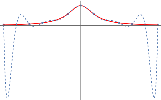
 is terrible! What’s going on? Why doesn’t polynomial interpolation work here? Can we fix it? The answer to the last question is yes and the solution is Chebyshev polynomials.

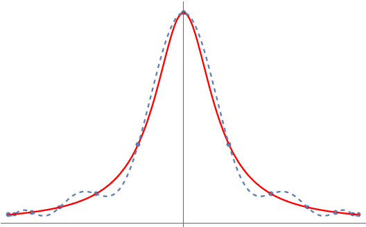
 , like this for ourselves. We’ll assume the interpolation points are given by a function
  so we can form the polynomial interpolant for any desired polynomial degree
  being \textit{injective} so that the points
  are guaranteed to be distinct.
 , the points look like this:
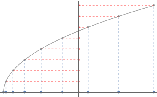

 (shown on horizontal axis)
 .
.
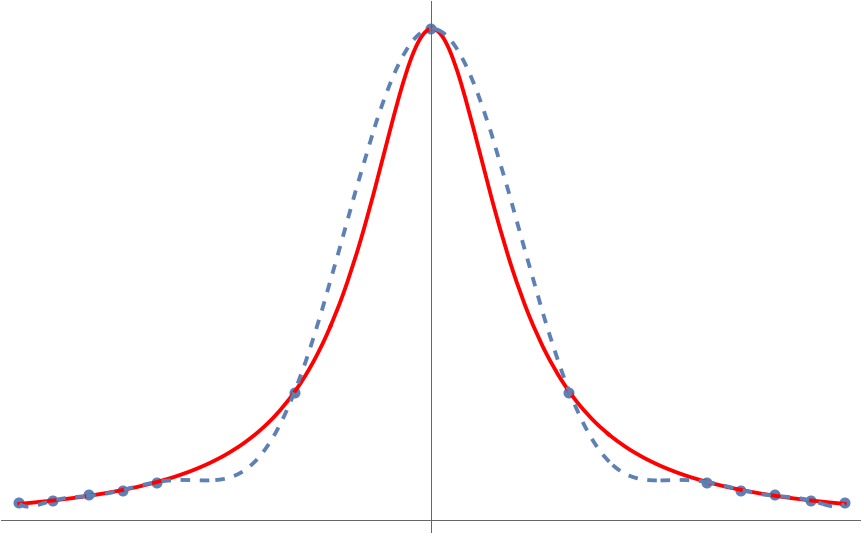
 , we see that these interpolation points now lead to a failure to approximate the function at the middle of the interval, even if we use a lot of interpolation points!
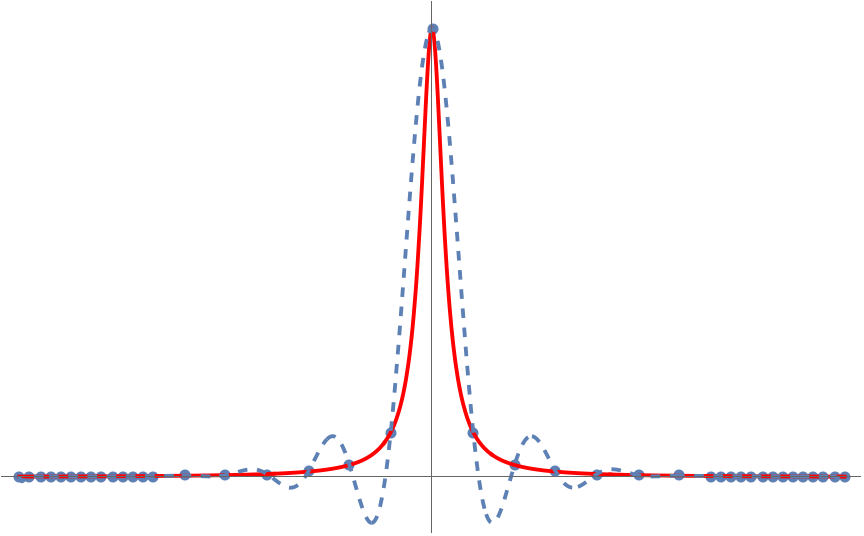
 and
and  are, the more clustered the points will be. For instance,


 , and
, and ,
,  .
. . This function yields points which are more clustered at the endpoints:


 which not too rough (i.e.,
  gives the
  radians along the unit circle. This means that the Chebyshev points are the
  ).
).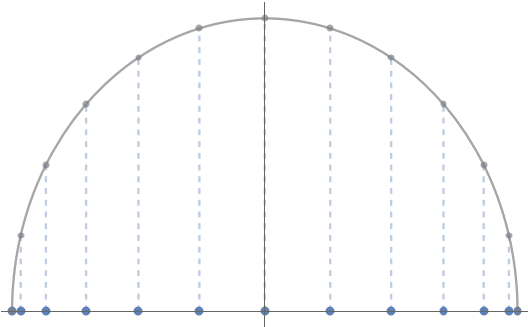
 look like as a function of the angle
  to
to 
 , is a polynomial in the variable
 always take the form

 units of frequency
  units of frequency
  units of frequency
  with exponentially small errors in the number of interpolation points used. By contrast, functions with kinks like
  are approximated with errors which decay much more slowly. See
 is
is  since multiple
  , between which the cosine function is
 , we’ve instead written
 are known as the
  are known as the Chebyshev polynomials
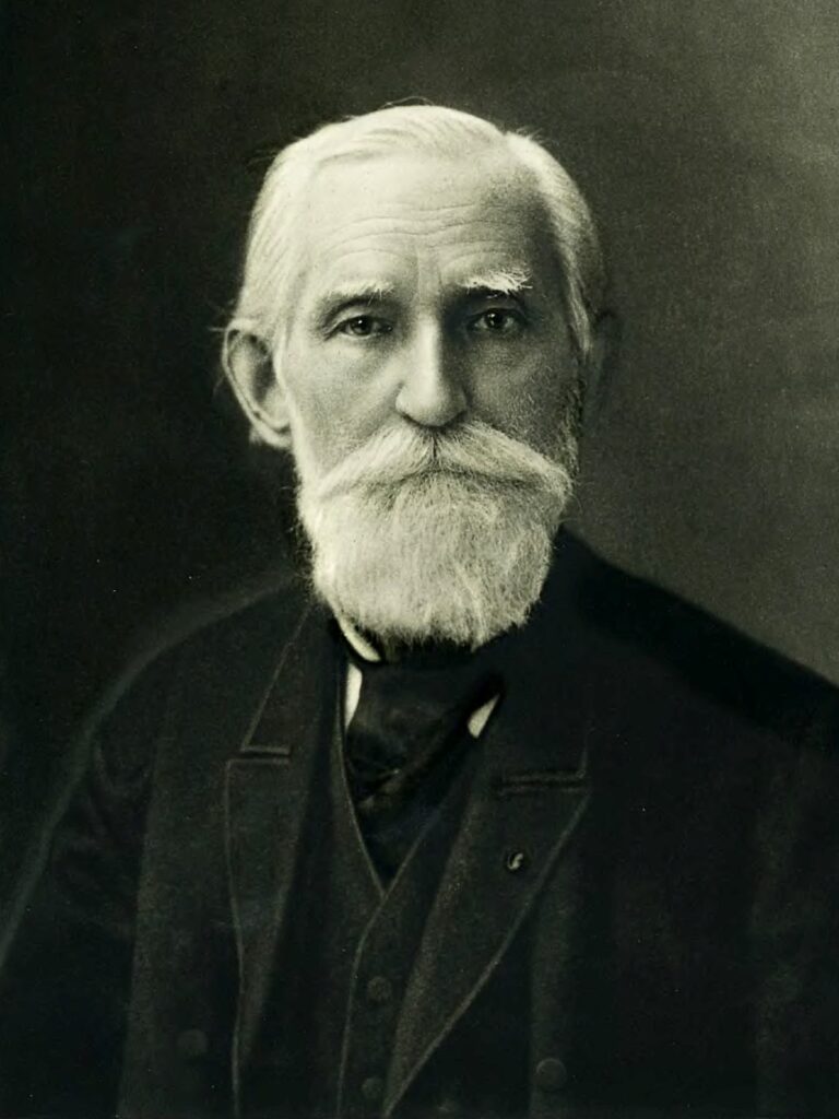

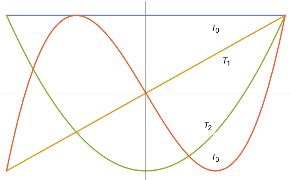
 for
for 
 and
and  are both polynomials, every Chebyshev polynomial is as well.
![\[p^\circ(\theta) = b_n\cos(n\theta) + \cdots + b_1\cos\theta + b_0\]](https://www.ethanepperly.com/wp-content/ql-cache/quicklatex.com-1c6828300bbae5fa0051e7c134da1d61_l3.png "Rendered by QuickLaTeX.com")
![\[p(x) = b_nT_n(x) + \cdots + b_1 T_1(x) + b_0.\]](https://www.ethanepperly.com/wp-content/ql-cache/quicklatex.com-cb291d9f73ebc4e74d0455dac4558a48_l3.png "Rendered by QuickLaTeX.com")
 are orthogonal to each other; are the Chebyshev polynomials?
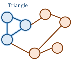
 triplets and checking whether they form a triangle is far too computationally costly for the billions of Facebook accounts. Somehow, we want to do much faster than this, and to achieve this speed we would be willing to settle for an estimate of the triangle count up to some error.
 matrix where the
  th entry of
  of the matrix
  where
where  , and
, and  , which is twice the number of triangles incident on
  and
and  are both counted as paths of length 3 for a triangle consisting of
  is counted thrice in the
  th, and
  th entries of
 for a vector
  . Therefore, the matrix
  , we simply compute matrix–vector products with
  .
. and
and  occurs with equal
  . Since the entries of
  and
and  are independent, the
  is
is  is
is![\begin{equation*} \mathbb{E} \, x^\top M x = \sum_{i,j=1}^n M_{ij} \mathbb{E} [x_ix_j] = \sum_{i = 1}^n M_{ii} = \operatorname{tr}(M). \end{equation*}](https://www.ethanepperly.com/wp-content/ql-cache/quicklatex.com-17a6a7cacc94a45f13853dc8f34f1e3a_l3.png "Rendered by QuickLaTeX.com")
 . Thus, the efficiently computable quantity
  equals
  and compute the averaged trace estimator
 remains an unbiased estimator for
  , but with reduced variability. Quantitatively, the
 .” In other words, concentration inequalities can provide quantitative estimates of the likely size of the error when a randomized algorithm is executed.
 is bounded by the expected value of
 . This small example shows both the power and the limitation of Markov’s inequality. On the negative side, our analysis suggests that we might have to wait as much as 100 times the average runtime for the algorithm to complete running with 99% probability; this large huge multiple of 100 seems quite pessimistic. On the other hand, we needed no information whatsoever about how the algorithm works to do this analysis. In general, Markov’s inequality cannot be improved without more assumptions on the random variable
  :
:
 denote the average

 . Therefore, by Chebyshev’s inequality,
 and are willing to tolerate a failure probability of
 . Normal random variables have an exponentially small probability of being more than a few standard deviations above their mean, so it is natural to expect this should be true of
 . Hoeffding’s inequality makes the assumption that the summands are bounded, say within an interval
 ![[a,b]](https://www.ethanepperly.com/wp-content/ql-cache/quicklatex.com-336bb22d4b2092329486008f6665b888_l3.png "Rendered by QuickLaTeX.com") .
.
 replaced by the potentially much larger quantity
 .
. for every
  . We continue to denote

 . We conclude that Bernstein’s inequality provides sharper bounds then Hoeffding’s inequality for smaller values of
  , except with failure probability at most

![[\mu-B,\mu+B]](https://www.ethanepperly.com/wp-content/ql-cache/quicklatex.com-bada0c6b976891e43bcc4c3b7508e96e_l3.png "Rendered by QuickLaTeX.com") for every
for every  , then
 samples are needed rather than proportional to
  . The fact that we need proportional to
  samples to achieve error
  to
to  , which is a huge improvement.
 ; for small values of
 is the
 . By the
  and
and  where
where  and
and  are the
  is the
  so
so  and
and  . Since the


 and
and  . Since we often don’t know good bounds for
  , one should really use the trace estimator together with an
  down from
  .
. is an
is an 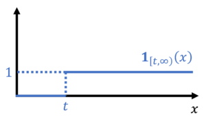
![\begin{equation*} \mathbb{P}\{X \ge t \} = \mathbb{E}[\mathbf{1}_{[t,\infty)}(X)]. \end{equation*}](https://www.ethanepperly.com/wp-content/ql-cache/quicklatex.com-070609e7e86c3846db2eec810355d5f4_l3.png "Rendered by QuickLaTeX.com")
 by bounding its corresponding indicator function. In particular, we have the inequality
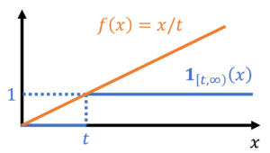
![\begin{equation*} \mathbb{P}\{ X \ge t \} = \mathbb{E}[\mathbf{1}_{[t,\infty)}(X)] \le \mathbb{E} \left[ \frac{X}{t} \right] = \frac{\mathbb{E} X}{t}. \end{equation*}](https://www.ethanepperly.com/wp-content/ql-cache/quicklatex.com-49a753eda4e591b364f5d4f3e24a0b9b_l3.png "Rendered by QuickLaTeX.com")

 by (11). To obtain sharp and useful bounds on
  we seek bounding functions
  ,
,  should be close to zero,
 ,
,  to be easily computable or boundable.
 or exponentials
  for which we have hopes of computing or bounding
  (by increasing
  , detracting from our ability to achieve point 2. We shall eventually come up with a best-possible resolution to this dilemma by formulating this as an optimization problem to determine the best choice of the parameter
  to obtain the best possible candidate function of the given form.
 satisfies the bound (13), and thus by (12),
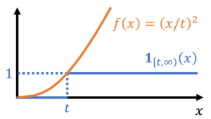
 , is a nonnegative random variable. Thus applying (14) gives
 if, and only if,
  . Therefore, by Markov’s inequality,
 , where

 ,
,  , and the
 up to the sign of the parameter
  . Taking logarithms proves the additivity.
 and consider the cumulant generating function of
  . Then one can show the cumulant generating function bound
 . We have
  . Since the function
  is
is  . Taking expectations, we have
  . One can show by comparing Taylor series that
  . Therefore, we have
  .
.


 :
:
 , we can apply a small trick. If we apply (20) to the summands
  instead of
 . The means of doing often this goes by the fancy name


 .
. matrix
  is as close to
  . That is, we seek to
 of
of  of
of  , our model predicts the output
  is approximately
  . The vector
  is as small as it could possibly be for all choices of coefficient vectors
 is invertible and the unique least squares solution to (1) is given by
  . We assume that
  and solve (2) using a linear solver like
  on a computer using a well-designed piece of software, one obtains an approximate solution
  which is, after accounting for the accumulation of rounding errors, close to
  .
. of the largest and smallest
 corresponds to the fact we have roughly 16 decimal digits of accuracy in double precision floating point arithmetic. Thus, if the condition number of
  , then we should expect around
  digits of accuracy in our computed solution.
 . We would hope that we can solve the least squares problem with an accuracy like the rule-of-thumb error bound (3) we had for linear systems of equations, namely a bound like
  . But this is not the kind of accuracy we get for the least squares problem when we solve it using the normal equations. Instead, we get accuracy like
 , then the normal equations give us absolute nonsense for
  times larger than
  . So even if we solve the least squares problem with QR factorization, we still get a squared condition number in our error bound, but this condition number squared is multiplied by the residual
  , which is small if the least squares fit is good. The least squares solution is usually only interesting when the residual is small, thus justifying dropping it in the rule of thumb.
 , etc.