Randomized Kaczmarz: How Should You Sample?

June 16, 2025 by Ethan N. Epperly Leave a comment

The randomized Kaczmarz method is a method for solving systems of linear equations:

(1) $\text{Find $x$ such that } Ax = b.$

Throughout this post, the matrix $A$ will have dimensions $n\times d$ . Beginning from an initial iterate $x_0 = 0$ , randomized Kaczmarz works as follows. For $t = 0,1,2,\ldots$ :

Sample a random row index $i_t$ with probability $\prob \{ i_t = j \} = p_j$ .
Update to enforce the equation $a_{i_t}^\top x = b_{i_t}$ holds exactly:
$x_{t+1} \coloneqq x_t + \frac{b_{i_t} - a_{i_t}^\top x_t}{\norm{a_{i_t}}^2} a_{i_t}.$
Throughout this post, $a_j^\top$ denotes the $j$ th row of $A$ .

What selection probabilities $p_j$ should we use? The answer to this question may depend on whether the system (1) is consistent, i.e., whether it possesses a solution $x$ . For this post, we assume (1) is consistent; see this previous post for a discussion of the inconsistent case.

The classical selection probabilities for randomized Kaczmarz were proposed by Strohmer and Vershynin in their seminal paper:

(1) $p_j = \frac{\norm{a_j}^2}{\norm{A}_{\rm F}^2} \quad \text{for } j = 1,2,\ldots,n.$

Computing these selection probabilities requires a full pass over the matrix, which can be expensive for the largest problems.¹ A computationally appealing alternative is to implement randomized Kaczmarz with uniform selection probabilities

(2) $p_j = \frac{1}{n} \quad \text{for } j = 1,2,\ldots,n.$

Ignoring computational cost, which sampling rule leads to faster convergence: (1) or (2)?

Surprisingly, to me at least, the simpler strategy (2) often works better than (1). Here is a simple example. Define a matrix $A \in \real^{20\times 20}$ with entries $A_{ij} = \min(i,j)^2$ , and choose the right-hand side $b\in\real^{20}$ with standard Gaussian random entries. The convergence of standard RK with sampling rule (1) and uniform RK with sampling rule (2) is shown in the plot below. After a million iterations, the difference in final accuracy is dramatic: the final relative error 0.00012 was uniform RK and 0.67 for standard RK!

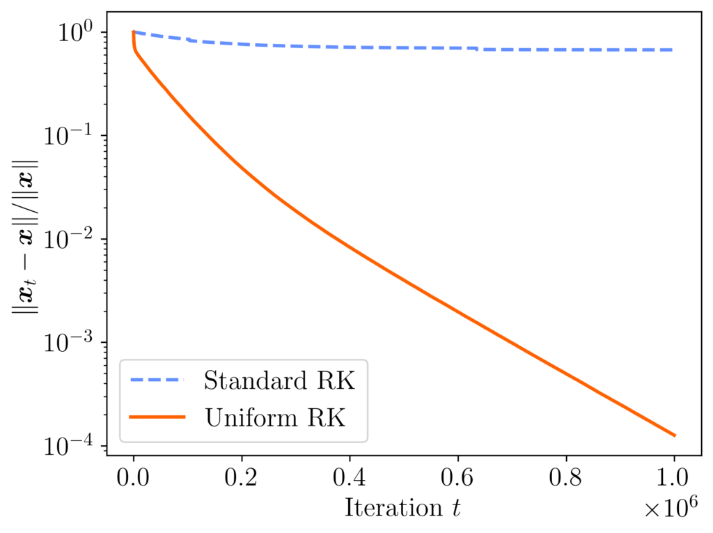
Error for randomized Kaczmarz with both squared row norm sampling ("standard") and uniformly random rows on matrix with entries min(i,j)^2. Uniform randomized Kaczmarz achieves significantly smaller final error

In fairness, uniform RK does not always outperform standard RK. If we change the matrix entries to $A_{ij} = \min(i,j)$ , then the performance of both methods is similar, with both methods ending with a relative error of about 0.07.

Error for randomized Kaczmarz with both squared row norm sampling ("standard") and uniformly random rows on matrix with entries min(i,j). Uniform randomized Kaczmarz and standard randomized Kaczmarz achieve comparable final errors

Another experiment, presented in section 4.1 of Strohmer and Vershynin’s original paper, provides an example where standard RK converges a bit more than twice as fast as uniform RK (called “simple RK” in their paper). Still, taken all together, these experiments demonstrate that standard RK (sampling probabilities (1)) is often not dramatically better than uniform RK (sampling probabilities (2)), and uniform RK can be much better than standard RK.

Randomized Kaczmarz Error Bounds

Why does uniform RK often outperform standard RK? To answer these questions, let’s look at the error bounds for the RK method.

The classical analysis of standard RK shows the method is geometrically convergent

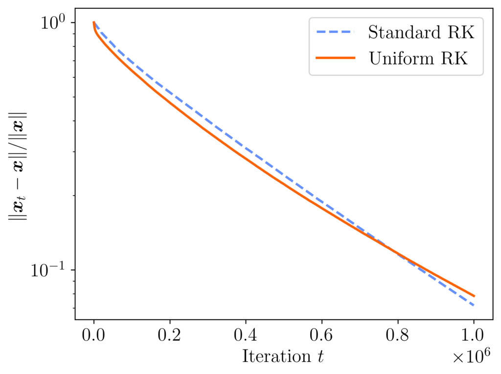
(3) $\expect\left[ \norm{x_t - x_\star}^2 \right] \le (1 - \kappa_{\rm dem}(A)^{-2})^t \norm{x_\star}^2.$

Here,

(4) $\kappa_{\rm dem}(A) = \frac{\norm{A}_{\rm F}}{\sigma_{\rm min}(A)} = \sqrt{\sum_i \left(\frac{\sigma_i(A)}{\sigma_{\rm min}(A)}\right)^2}$

is known as the Demmel condition number and $\sigma_i(A)$ are the singular values of $A$ . Recall that we have assumed the system $Ax = b$ is consistent, possessing a solution $x_\star$ . If there are multiple solutions, we let $x_\star$ denote the solution of minimum norm.

What about uniform RK? Let $D_A = \diag ( \norm{a_i}^{-1} : i=1,\ldots,n )$ denote a diagonal matrix containing the inverse row norms, and introduce the row-equilibrated matrix $D_A A$ . The row-equilibrated matrix $D_A A$ has been obtained from $A$ by rescaling each of its rows to have unit norm.

Uniform RK can then be related to standard RK run on the row-equilibrated matrix:

Fact (uniform sampling and row equilibration): Uniform RK on the system $Ax = b$ produces the same sequence of (random) iterates $\hat{x}_t$ as standard RK applied to the row-equilibrated system $(D_A A)x = D_A b$ .

Therefore, by (3), the iterates $\hat{x}_t$ of uniform RK satisfy the bound

(5) $\expect\left[ \norm{\hat{x}_t - x_\star}^2 \right] \le (1 - \kappa_{\rm dem}(D_A A)^{-2})^t \norm{x_\star}^2.$

Thus, at least using the error bounds (3) and (5), whether standard or uniform RK is better depends on which matrix has a smaller Demmel condition number: $A$ or $D_A A$ .

Row Equilibration and the Condition Number

Does row equilibration increase or decrease its condition number? What is the optimal way of scaling the rows of a matrix to minimize its condition number? These are classical questions in numerical linear algebra, and they were addressed in a classical 1969 paper of van der Sluis. These results were then summarized and generalized in Higham’s delightful monograph Accuracy and Stability of Numerical Algorithms. Here, we present answers to these questions using a variant of van der Sluis’ argument.

First, let’s introduce some more concepts and notation. Define the spectral norm condition number

$\kappa(A) \coloneqq \frac{\sigma_{\rm max}(A)}{\sigma_{\rm min}(A)}$

The spectral norm and Demmel condition numbers are always comparable $\kappa(A) \le \kappa_{\rm dem}(A)\le \sqrt{\min(n,d)}\cdot \kappa(A)$ . Also, let $\mathrm{Diag}$ denote the set of all (nonsingular) diagonal matrices.

Our first result shows us that row equilibration never hurts the Demmel condition number by much. In fact, the row-equilibrated matrix produces a nearly optimal Demmel condition number when compared to any row scaling:

Theorem 1 (Row equilibration is a nearly optimal row scaling). Let $A\in\real^{n\times d}$ be wide $n\le d$ and full-rank, and let $D_AA$ denote the row-scaling of $A$ to have unit row norms. Then
$\kappa_{\rm dem}(D_AA) \le \sqrt{n}\cdot \min_{D \in \mathrm{Diag}} \kappa (DA) \le \sqrt{n}\cdot \min_{D \in \mathrm{Diag}} \kappa_{\rm dem} (DA).$

By scaling the rows of a square or wide matrix to have unit norm, we bring the Demmel condition number to within a $\sqrt{n}$ factor of the optimal row scaling. In fact, we even bring the Demmel condition number to within a $\sqrt{n}$ factor of the optimal spectral norm condition number for any row scaling.

Since the convergence rate for randomized Kaczmarz is $\kappa_{\rm dem}(A)^{-2}$ , this result shows that implementing randomized Kaczmarz with uniform sampling yields to a convergence rate that is within a factor of $n$ of the optimal convergence rate using any possible sampling distribution.

This result shows us that row equilibration can’t hurt the Demmel condition number by much. But can it help? The following proposition shows that it can help a lot for some problems.

Proposition 2 (Row equilibration can help a lot). Let $A\in\real^{n\times d}$ be wide $n\le d$ and full-rank, and let $\gamma$ denote the maximum ratio between two row norms:
$\gamma \coloneqq \frac{ \max_i \norm{a_i}}{\min_i \norm{a_i}}.$
Then the Demmel condition number of the original matrix $A$ satisfies
$\kappa_{\rm dem}(A) \le \gamma \cdot \kappa_{\rm dem}(D_A A).$
Moreover, for every $\gamma\ge 1$ , there exists a matrix $A_\gamma$ where this bound is nearly attained:
$\kappa_{\rm dem}(A_\gamma) \ge \sqrt{1-\frac{1}{n}} \cdot \gamma \cdot \kappa_{\rm dem}(D_{A_\gamma}A_\gamma).$

Taken together, Theorem 1 and Proposition 2 show that row equilibration often improves the Demmel condition number, and never increases it by that much. Consequently, uniform RK often converges faster than standard RK for square (or short wide) linear systems, and it never converges much slower.

Proof of Theorem 1

We follow Higham’s approach. Each of the $n$ rows of $D_AA$ each have unit norm, so

(7) $\norm{D_AA}_{\rm F} = \sqrt{n}.$

The minimum singular value of $D_A A$ can be written in terms of the Moore–Penrose pseudoinverse $(D_A A)^\dagger = A^\dagger D_A^{-1}$ as follows

$\frac{1}{\sigma_{\rm min}(D_A A)} = \norm{A^\dagger D_A^{-1}}.$

Here, $\norm{\cdot}$ denotes the spectral norm. Then for any nonsingular diagonal matrix $D$ , we have

(8) $\frac{1}{\sigma_{\rm min}(D_A A)} = \norm{A^\dagger D^{-1} (DD_A^{-1})} \le \norm{A^\dagger D^{-1}} \norm{DD_A^{-1}} = \frac{\norm{DD_A^{-1}}}{\sigma_{\rm min}(DA)}.$

Since the matrix $DD_A^{-1}$ is diagonal its spectral norm is

$\norm{DD_A^{-1}} = \max \left\{ \frac{|D_{ii}|}{|(D_A)_{ii}|} : 1\le i \le n \right\}.$

The diagonal entries of $D_A$ are $\norm{a_i}^{-1}$ , so

$\norm{DD_A^{-1}} = \max \left\{ |D_{ii}|\norm{a_i} : 1\le i\le n \right\}$

is the maximum row norm of the scaled matrix $DA$ . The maximum row norm is always less than the largest singular value of $DA$ , so $\norm{DD_A^{-1}} \le \sigma_{\rm max}(DA)$ . Therefore, combining this result, (7), and (9), we obtain

$\kappa_{\rm dem}(D_AA) \le \sqrt{n} \cdot \frac{\sigma_{\rm max}(DA)}{\sigma_{\rm min}(DA)} = \sqrt{n}\cdot \kappa (DA).$

Since this bound holds for every $D \in \mathrm{Diag}$ , we are free to minimize over $D$ , leading to the first inequality in the theorem:

$\kappa_{\rm dem}(D_AA) \le \sqrt{n}\cdot \min_{D \in \mathrm{Diag}} \kappa (DA).$

Since the spectral norm condition number is smaller than the Demmel condition number, we obtain the second bound in the theorem.

Proof of Proposition 2

Write $A = D_A^{-1}(D_AA)$ . Using the Moore–Penrose pseudoinverse again, write

(10) $\kappa_{\rm dem}(A) = \norm{D_A^{-1}(D_AA)}_{\rm F} \norm{(D_A A)^\dagger D_A}.$

The Frobenius norm and spectral norm satisfy a (mixed) submultiplicative property

$\norm{BC}_{\rm F} \le \norm{B}\norm{C}_{\rm F}, \quad \norm{BC} \le\norm{B}\norm{C}.$

Applying this result to (1), we obtain

$\kappa_{\rm dem}(A) \le \norm{D_A^{-1}}\norm{D_AA}_{\rm F} \norm{(D_A A)^\dagger} \norm{D_A}.$

We recognize $\gamma = \norm{D_A^{-1}}\norm{D_A}$ and $\kappa_{\rm dem}(D_A A) = \norm{D_AA}_{\rm F} \norm{(D_A A)^\dagger}$ . We conclude

$\kappa_{\rm dem}(A) \le \gamma \cdot \kappa_{\rm dem}(D_A A).$

To show this bound is nearly obtained, introduce $A_\gamma = \diag(\gamma,\gamma,\ldots,\gamma,1)$ . Then $D_{A_\gamma} A_\gamma = I$ with $\kappa_{\rm dem}(D_{A_\gamma}A_{\gamma}) = \sqrt{n}$ and

$\kappa_{\rm dem}(A_\gamma) = \frac{\norm{A_{\gamma}}_{\rm F}}{\sigma_{\rm min}(A_\gamma)} = \frac{\sqrt{(n-1)\gamma^2+1}}{1} \ge \sqrt{n} \cdot \sqrt{1-\frac{1}{n}} \cdot \gamma.$

Therefore,

$\kappa_{\rm dem}(A_\gamma) \ge \sqrt{1-\frac{1}{n}} \cdot \gamma \cdot \kappa_{\rm dem}(D_{A_\gamma}A_\gamma).$

Practical Guidance

What does this theory mean for practice? Ultimately, single-row randomized Kaczmarz is often not the best algorithm for the job for ordinary square (or short–wide) linear systems, anyway—block Kaczmarz or (preconditioned) Krylov methods have been faster in my experience. But, supposing that we have locked in (single-row) randomized Kaczmarz as our algorithm, how should we implement it?

This question is hard to answer, because there are examples where standard RK and uniform RK both converge faster than the other. Theorem 1 suggests uniform RK can require as many as $n\times$ more iterations than standard RK on a worst-case example, which can be a big difference for large problems. But, particularly for badly row-scaled problems, Proposition 2 shows that uniform RK can dramatically outcompete standard RK. Ultimately, I would give two answers.

First, if the matrix $A$ has already been carefully designed to be well-conditioned and computing the row norms is not computationally burdensome, then standard RK may be worth the effort. Despite this theory suggesting it can do quite badly, it took a bit of effort to construct a simple example of a “bad” matrix where uniform RK significantly outcompeted standard RK. (On most examples I constructed, the rate of convergence of the two methods were similar.)

Second, particularly for the largest systems where you only want to make a small number of total passes over the matrix, expending a full pass over the matrix to compute the row norms is a significant expense. And, for poorly row-scaled matrices, sampling using the squared row norms can hurt the convergence rate. Based on these observations, given a matrix of unknown row scaling and conditioning or given a small budget of passes over the matrix, I would use the uniform RK method over the standard RK method.

Finally, let me again emphasize that the theoretical results Theorem 1 and Proposition 2 only apply to square or wide matrices $A$ . Uniform RK also appears to work for consistent systems with a tall matrix, but I am unaware of a theoretical result comparing the Demmel condition numbers of $D_AA$ and $A$ that applies to tall matrices. And for inconsistent systems of equations, it’s a whole different story.

Edit: After initial publication of this post, Mark Schmidt shared that the observation that uniform RK can outperform standard RK was made nearly ten years ago in section 4.2 of the following paper. They support this observation with a different mathematical justification

The Schur Product Theorem

February 25, 2025 by Ethan N. Epperly Leave a comment

The Schur product theorem states that the entrywise product $A\circ M$ of two positive semidefinite matrices is also positive semidefinite. This post will present every proof I know for this theorem, and I intend to edit it to add additional proofs if I learn of them. (Please reach out if you know another!) My goal in this post is to be short and sweet, so I will assume familiarity with many properties for positive semidefinite matrices.

For this post, a matrix $A\in\real^{n\times n}$ is positive semidefinite (psd, for short) if it is symmetric and satisfies $x^\top Ax\ge 0$ for all vectors $x\in\real^n$ . All matrices in this post are real, though the proofs we’ll consider also extend to complex matrices. The entrywise product will be denoted $\circ$ and is defined as $(A\circ M)_{ij} = A_{ij}M_{ij}$ . The entrywise product is also known as the Hadamard product or Schur product.

It is also true that the entrywise product of two positive definite matrices is positive definite. The interested reader may be interested in seeing which of the proofs also yield this result.

Proof 1: Trace formula

We start by computing $x^\top (A\circ M)x$ :

$x^\top (A\circ M)x = \sum_{i,j=1}^n x_i (A\circ M)_{ij} x_j = \sum_{i,j=1}^n x_i A_{ij} M_{ij} x_j.$

Now, we may rearrange the sum, use symmetry of $M$ , and repackage it as a trace

$x^\top (A\circ M)x = \sum_{i,j=1}^n x_i A_{ij} x_j M_{ji} = \tr(\operatorname{diag}(x) A \operatorname{diag}(x) M).$

This the trace formula for quadratic forms in the Schur product.

Recall that a matrix $A$ is psd if and only if it $A$ is a Gram matrix (able to be expressed as $A = B^\top B$ ). Thus, we may write $A = B^\top B$ and $M = C^\top C$ . Substituting these expressions in the trace formula and invoking the cyclic property of the trace, we get

$x^\top (A\circ M)x = \tr(\operatorname{diag}(x) B^\top B \operatorname{diag}(x) C^\top C) = \tr(C\operatorname{diag}(x) B^\top B \operatorname{diag}(x) C^\top).$

The matrix on the right-hand side has the expression

$C\operatorname{diag}(x) B^\top B \operatorname{diag}(x) C^\top = G^\top G \quad \text{for } G = B \operatorname{diag}(x) C^\top.$

Therefore, it is psd and so its trace is psd:

$x^\top (A\circ M)x = \tr(G^\top G) \ge 0.$

We have shown $x^\top (A\circ M)x\ge 0$ for every vector $x$ , so $A\circ M$ is psd.

Proof 2: Gram matrix

Since $A$ and $M$ are psd, they may be written as $A = B^\top B$ and $M = C^\top C$ . Letting $b_i^\top$ and $c_i^\top$ denote the $i$ th rows of $B$ and $C$ , we have

$A = \sum_i b_ib_i^\top \quad \text{and} \quad M = \sum_j c_jc_j^\top.$

Computing the Schur product and distributing, we have

$A\circ M = \sum_{i,j} (b_ib_i^\top \circ c_jc_j^\top).$

The Schur product of rank-one matrices $b_ib_i^\top$ and $c_jc_j^\top$ is, by direct computation, $(b_i\circ c_j)(b_i\circ c_j)^\top$ . Thus,

$A\circ M = \sum_{i,j} (b_i\circ c_j)(b_i\circ c_j)^\top$

is a sum of (rank-one) psd matrices and is thus psd.

Proof 3: Covariances

Let $x$ and $y$ be independent random vectors with zero mean and covariance matrices $A$ and $M$ . The vector $x\circ y$ is seen to have zero mean as well. Thus, the $ij$ entry of the covariance matrix $\Cov(x\circ y)$ of $x\circ y$ is

$\expect[x_iy_ix_jy_j] = \expect[x_ix_j] \expect[y_iy_j] = A_{ij} M_{ij} = (A\circ M)_{ij}.$

The second equality is the independence of $x$ and $y$ , and the third equality uses the fact that $A$ and $M$ are the covariance matrices of $x$ and $y$ . Thus, the covariance matrix of $x\circ y$ is $A\circ M$ . All covariance matrices are psd, so $A\circ M$ is psd as well.¹

Proof 4: Kronecker product

The Kronecker product $A\otimes M$ of two psd matrices is psd. The entrywise product $A\circ M$ is a principal submatrix of $A\otimes M$ :

$A\circ M = ((A\otimes M)_{(i+n(i-1))(i+n(i-1))} : i = 1,\ldots,n).$

All principal submatrices of a psd matrix are psd, so $A\circ M$ is psd.

My Favorite Proof of the Cauchy–Schwarz Inequality

December 10, 2024 by Ethan N. Epperly 2 Comments

The Cauchy–Schwarz inequality has many proofs. Here is my favorite, taken from Chapter 3 of The Schur complement and its applications; the book is edited by Fuzhen Zhang, and this chapter was contributed by him as well. Let $x,y \in \real^n$ be vectors, assemble the matrix $B = \onebytwo{x}{y}$ , and form the Gram matrix

$A = B^\top B = \onebytwo{x}{y}^\top \onebytwo{x}{y} = \twobytwo{\norm{x}^2}{y^\top x}{x^\top y}{\norm{y}^2}.$

Since $A$ is a Gram matrix, it is positive semidefinite. Therefore, its determinant is nonnegative:

$\det(A) = \norm{x}^2\norm{y}^2 - |x^\top y|^2 \ge 0.$

Rearrange to obtain the Cauchy–Schwarz inequality

$|x^\top y| \le \norm{x}\norm{y}.$

Equality occurs if and only if $A$ is a rank-one matrix, which occurs if and only if $x$ and $y$ are scalar multiples.

I like this proof because it is perhaps the simplest example of the (block) matrix technique for proving inequalities. Using this technique, one proves inequalities about scalars (or matrices) by embedding them in a clever way into a (larger) matrix. Here is another example of the matrix technique, adapted from the proof of Theorem 12.9 of these lecture notes by Joel Tropp. Jensen’s inequality is a far-reaching and very useful inequality in probability theory. Here is one special case of the inequality.

Proposition (Jensen’s inequality for the inverse): Let $x_1,\ldots,x_n$ be strictly positive numbers. Then the inverse of their average is no bigger than the average of their inverses:
$\left( \frac{1}{n} \sum_{i=1}^n x_i \right)^{-1} \le \frac{1}{n} \sum_{i=1}^n \frac{1}{x_i}.$

To prove this result, embed each $x_i$ into a $2\times 2$ positive semidefinite matrix $\twobytwo{x_i}{1}{1}{1/x_i}$ . Taking the average of all such matrices, we observe that

$A = \twobytwo{\frac{1}{n} \sum_{i=1}^n x_i}{1}{1}{\frac{1}{n} \sum_{i=1}^n \frac{1}{x_i}}$

is positive semidefinite as well. Thus, its determinant is nonnegative:

$\det(A) = \left(\frac{1}{n} \sum_{i=1}^n x_i\right) \left(\frac{1}{n} \sum_{i=1}^n \frac{1}{x_i}\right) - 1 \ge 0.$

Rearrange to obtain

$\left( \frac{1}{n} \sum_{i=1}^n x_i \right)^{-1} \le \frac{1}{n} \sum_{i=1}^n \frac{1}{x_i}.$

Remarkably, we have proven a purely scalar inequality by appeals to matrix theory.

The matrix technique for proving inequalities is very powerful. Check out Chapter 3 of The Schur complement and its applications for many more examples.

If you like this blog and want another way to follow it, I am starting newsletter:

Rejection Sampling

October 8, 2024 by Ethan N. Epperly 4 Comments

I am delighted to share that my paper Embrace rejection: Kernel matrix approximation with randomly pivoted Cholesky has been released on arXiv, joint with Joel Tropp and Rob Webber.

On the occasion of this release, I want to talk about rejection sampling, one of the most powerful ideas in probabilistic computing. My goal is to provide an accessible and general introduction to this technique, with a more “applied math” rather than statistical perspective. I will conclude with some discussion of how we use it in our paper.

Motivating Application: Randomized Kaczmarz

Consider the task of solving a linear system of equations $Ax = b$ , where $A \in \real^{n\times d}$ is a matrix and $b \in \real^n$ is a vector. For simplicity, we assume that this system is consistent (i.e., there exists a solution $x_\star$ such that $Ax_\star = b$ ). The randomized Kaczmarz algorithm is a mathematically elegant algorithm for solving this problem, due to Strohmer and Vershynin. Beginning with initial solution $x \gets 0$ , randomized Kaczmarz repeatedly performs the following steps:

Sample. Generate a random row index $I$ according to the probability distribution $\prob \{I = i\} = \norm{a_i}^2 / \norm{A}_{\rm F}^2$ . Here, and going forward, $a_i^\top$ denotes the $i$ th row of $A$ and $\norm{\cdot}_{\rm F}$ is the Frobenius norm.
Update. Set $x \gets x + (b_I - a_I^\top x)\cdot a_I / \norm{a_I}^2$ .

Convergence theory of the randomized Kaczmarz iteration is very well-studied; see, e.g., section 4.1 of this survey for an introduction.

For this post, we will consider a more basic question: How can we perform the sampling step 1? If $n$ and $d$ are not very large, this is an easy problem: Simply sweep through all the rows $a_i$ and compute their norms $\norm{a_i}^2$ . Then, sampling can be done using any algorithm for sampling from a weighted list of items. But what if $n$ is very large? Suppose, even, that it is computationally expensive to read through the matrix, even once, to compute the row norms. What can we do now?

Here is one solution is using rejection sampling, due to Needell, Ward, and Srebro. Suppose that we know a bound on the row norms of $A$ :

(1) $\norm{a_i}^2 \le B \quad \text{for each } i = 1,\ldots,n.$

For instance, if the entries of $A$ take values in the range $[-1,1]$ , then (1) holds with $B = d$ . To sample a row $i$ with probability $\norm{a_i}^2/\norm{A}_{\rm F}^2$ , we perform the following the rejection sampling procedure:

Propose. Draw a random row index $1\le J\le n$ uniformly at random (i.e., $J$ is equally likely to be any row index between $1$ and $n$ .)
Accept/reject. Make a random choice: With probability $p_J = \norm{a_J}^2/B$ , accept and set $I\gets J$ . With the remaining probability $1-p_J$ , reject and return to step 1.

Why does this procedure work? As an intuitive explanation, notice that each row $i$ is equally likely to be proposed and has probability proportional to $\norm{a_i}^2$ of being accepted. Therefore, under this procedure, each row $i$ has probability proportional to $\norm{a_i}^2$ of being selected, just as desired for randomized Kaczmarz. If this intuitive justification is unsatisfying, we’ll have a formal derivation of correctness below (in a more general context).

I find rejection sampling to be super neat. In this case, it allows us to use simple ingredients (uniform row sampling and an upper bound on the row norms) to accomplish a more complicated task (sampling according to the squared row norms). We can sample from an interesting probability distribution (the squared row norm distribution) by thinning out samples from a simple distribution. This is a powerful idea that has many applications. (And, I believe, many more applications are waiting to be discovered.)

Rejection Sampling in General

Let’s now discuss rejection sampling in a bit more generality. Say I have a list of $n$ things each of which has a weight $w_i\ge 0$ . Our goal is to choose a random index $I$ with probability proportional to $w_i$ , i.e., $\prob \{ I = i\} = w_i / \sum_{j=1}^n w_j$ . We will call $w$ the target distribution. (Note that we do not require the weights $w_i$ to be normalized to satisfy $\sum_{i=1}^n w_i =1$ .)

Suppose that sampling from the target distribution is challenging, but we can sample from a proposal distribution $\rho$ , i.e., we can efficiently generate random $J$ such that $\prob \{J = i\} = \rho_i / \sum_{j=1}^n \rho_j$ . Further, suppose that the proposal distribution dominates the target distribution in the sense that

$w_i \le \rho_i \quad \text{for each } i=1,\ldots,n.$

Under this general setting, we can sample $I$ from the target distribution using rejection sampling, similar to above:

Propose. Draw a random row index $J$ from the proposal distribution.
Accept/reject. Make a random choice: With probability $p_J = w_J/\rho_J$ , accept and set $I\gets J$ . With the remaining probability $1-p_J$ , reject and return to step 1.

We recognize the squared row-norm sampling above as an example of this general strategy with $w_i = \norm{a_i}^2$ and $\rho_i = B$ for all $i$ .

Let us now convince ourselves more carefully that rejection sampling works. On any given execution of the rejection sampling loop, the probability of proposing index $i$ is $\rho_i / \sum_{j=1}^n \rho_j$ , after which the probability of accepting $i$ is $w_i / \rho_i$ . Therefore, the probability of outputting $i$ at any given loop is

$\prob \{\text{$i$ accepted this loop}\} = \frac{\rho_i}{\sum_{j=1}^n \rho_j} \cdot \frac{w_i}{\rho_i} = \frac{w_i}{\sum_{j=1}^n \rho_j}.$

The probability that any index $i$ on that loop is accepted is thus

$\prob \{\text{any accepted this loop}\} = \sum_{i=1}^n \prob \{\text{$i$ accepted this loop}\} = \frac{\sum_{i=1}^n w_i}{\sum_{i=1}^n \rho_i}.$

The rejection sampling loop accepts with fixed positive probability each execution, so it eventually accepts with 100% probability. Thus, the probability of accepting $i$ conditional on some index being accepted is

$\prob \{\text{$i$ accepted this loop} \mid \text{any accepted this loop}\} = \frac{\prob \{\text{$i$ accepted this loop}\}}{\prob \{\text{any accepted this loop}\}} = \frac{w_i}{\sum_{j=1}^n w_j}.$

Therefore, rejection sampling outputs a sample $I$ from the target distribution $w$ as promised.

As this analysis shows, the probability of accepting on any given execution of the rejection sampling loop is $\sum_{i=1}^n w_i / \sum_{i=1}^n \rho_i$ , the ratio of the total mass of the target $w_i$ to the total mass of the proposal $\rho_i$ . Thus, rejection sampling will have a high acceptance rate if $w_i \approx \rho_i$ and a low acceptance rate if $w_i \ll \rho_i$ . The conclusion for practice is that rejection sampling is only computationally efficient if one has access to a good proposal distribution $\rho_i$ , that is both easy to sample from and close to the target $w_i\approx \rho_i$ .

Here, we have presented rejection sampling as a strategy for sampling from a discrete set of items $i=1,\ldots,n$ , but this not all that rejection sampling can do. Indeed, one can also use rejection sampling for sampling a real-valued parameters $x \in \real$ or a multivariate parameter $x \in \real^n$ from a given (unnormalized) probability density function (or, if one likes, an unnormalized probability measure).

Before moving on, let us make one final observation. A very convenient thing about rejection sampling is that we only need the unnormalized probability weights $w_i$ and $\rho_i$ to implement the procedure, even though the total weights $\sum_{j=1}^n w_i$ and $\sum_{j=1}^n \rho_i$ are necessary to define the sampling probabilities $\prob \{I = i\} = w_i / \sum_{j=1}^n w_j$ and $\prob \{J = i\} = \rho_i / \sum_{j=1}^n \rho_j$ . This fact is necessary for many applications of rejection sampling. For instance, in the randomized Kaczmarz use, rejection sampling would be much less useful if we needed the total weight $\sum_{i=1}^n \norm{a_i}^2 = \norm{A}_{\rm F}^2$ , as computing $\norm{A}_{\rm F}^2$ requires a full pass over the data to compute.

Application: Randomly pivoted Cholesky

Another application of rejection sampling appears is to accelerate the randomly pivoted Cholesky algorithm, the subject of my recent paper. Here, I’ll provide an overview of the main idea with a focus on the role of rejection sampling in the procedure. See the paper for more details. Warning: Even as simplified here, this section presents a significantly more involved application of rejection sampling than we saw previously with randomized Kaczmarz!

Randomly pivoted Cholesky (RPCholesky) is a simple, but powerful algorithm for computing a low-rank approximation to a symmetric positive semidefinite matrix $A$ , and it can be used to accelerate kernel machine learning algorithms.

Conceptually, RPCholesky works as follows. Let $A^{(0)} \coloneqq A$ denote the initial matrix and $\hat{A}^{(0)} \coloneqq 0$ denote a trivial initial approximation. For $j=0,1,2,\ldots,k-1$ , RPCholesky performs the following steps:

Random sampling. Draw a random index $I_{j+1}$ with probability $\prob \{ I_{j+1} = i\} = A^{(j)}_{ii} / \sum_{i=1}^n A^{(j)}_{ii}$ .
Update approximation. Update $\hat{A}^{(j+1)} \gets \hat{A}^{(j)} + a_i^{(j)}(a_i^{(j)})^\top / A_{ii}^{(j)}$ . Here, $a_i^{(j)}$ denotes the $i$ th column of $A^{(j)}$ .
Update matrix. Update $A^{(j+1)} \gets A^{(j)} + a_i^{(j)}(a_i^{(j)})^\top / A_{ii}^{(j)}$ .

The result of this procedure is a rank- $k$ approximation $\hat{A}^{(k)}$ . With an optimized implementation, RPCholesky requires only $O(k^2N)$ operations and evaluates just $(k+1)N$ entries of the input matrix $A$ .

The standard RPCholesky algorithm is already fast, but there is room for improvement. The standard RPCholesky method processes the matrix $A$ one column $a_i$ at a time, but modern computers are faster at processing blocks of columns. Using the power of rejection sampling, we can develop faster versions of RPCholesky that take advantage of blocked computations. These blocked implementations are important: While we could handle a million-by-million matrix using the standard RPCholesky method, blocked implementations can be up to 40 $\times$ faster. In this post, I’ll describe the simplest way of using rejection sampling to implement RPCholesky.

To set the stage, let’s first establish some notation and make a few observations. Let $S_j = \{I_1,\ldots,I_j\}$ denote the first $j$ selected random indices. With a little matrix algebra, one can show that the approximation $\hat{A}^{(j)}$ produced by $j$ steps of RPCholesky obeys the formula¹

(1) $\hat{A}^{(j)} = A(:,S_j) A(S_j,S_j)^{-1}A(S_j,:).$

Here, we are using MATLAB notation for indexing the matrix $A$ . The residual matrix $A^{(j)}$ is given by

$A^{(j)} = A - \hat{A}^{(j)} = A - A(:,S_j) A(S_j,S_j)^{-1}A(S_j,:).$

Importantly for us, observe that we can evaluate the $i$ th diagonal entry of $A^{(j)}$ using the formula

(2) $A^{(j)}_{ii} = A_{ii} - A(i,S_j) A(S_j,S_j)^{-1} A(S_j,i).$

Compared to operating on the full input matrix $A$ , evaluating an entry $A^{(j)}_{ii}$ is cheap, just requiring some arithmetic involving matrices and vectors of size $j$ .

Here, we see a situation similar to randomized Kaczmarz. At each step of RPCholesky, we must sample a random index $I_{j+1}$ from a target distribution $w_i = A_{ii}^{(j)}$ , but it is expensive to evaluate all of the $w_i$ ‘s. This is a natural setting for rejection sampling. As proposal distribution, we may use the initial diagonal of $A$ , $\rho_i = A_{ii}$ . (One may verify that, as required, $w_i = A_{ii}^{(j)} \le A_{ii} = \rho_i$ for all $i$ .) This leads to a rejection sampling implementation for RPCholesky:

Sample indices. For $j=0,1,\ldots,k-1$ , sample random indices $I_{j+1}$ from the target distribution $w_i = A^{(j)}_{ii}$ using rejection sampling with proposal distribution $\rho_i = A_{ii}$ . Entries $A_{ii}^{(j)}$ are evaluated on an as-needed basis using (2).
Build the approximation. Form the approximation $\hat{A}^{(k)}$ all at once using (1).

By using rejection sampling, we have gone from an algorithm which handles the matrix one column at a time to a new algorithm which processes columns of the matrix $A$ all at once through the formula (1). In the right situations, this new algorithm can be significantly faster than the original RPCholesky method.²

We have now seen two extreme cases: the standard RPCholesky algorithm that processes the columns of $A$ one at a time and a rejection sampling implementation that operates on the columns of $A$ all at once. In practice, the fastest algorithm sits between these extremes, using rejection sampling to sample column indices in moderate-size blocks (say, between 100 and 1000 columns at a time). This “goldilocks” algorithm is the accelerated RPCholesky method that we introduce in our paper. Check it out for details!

Conclusion: Rejection Sampling, an Algorithm Design Tool

We’ve now seen two applications, randomized Kaczmarz and randomly pivoted Cholesky, where rejection sampling can be used to speed up an algorithm. In both cases, we wanted to sample from a distribution over $n$ row or column indices, but it was expensive to perform a census to compute the probability weight of each item individually. Rejection sampling offers a different approach, where we generate samples from a cheap-to-sample proposal distribution and only evaluate the probability weights of the proposed items. In the right situations, this rejection sampling approach can lead to significant computational speedups.

Rejection sampling has been used by statistics-oriented folks for decades, but the power of this technique seems less well-known to researchers in applied math, scientific computation, and related areas. I think there are a lot more exciting ways that we can use rejection sampling to design better, faster randomized algorithms.

Neat Randomized Algorithms: RandDiag for Rapidly Diagonalizing Normal Matrices

July 2, 2024 by Ethan N. Epperly Leave a comment

Consider two complex-valued square matrices $A\in\complex^{n\times n}$ and $B\in\complex^{n\times n}$ . The first matrix $A$ is Hermitian, being equal $A = A^*$ to its conjugate transpose $A^*$ . The other matrix $B$ is non-Hermitian, $B \ne B^*$ . Let’s see how long it takes to compute their eigenvalue decompositions in MATLAB:

>> A = randn(1e3) + 1i*randn(1e3); A = (A+A')/2;
>> tic; [V_A,D_A] = eig(A); toc % Hermitian matrix
Elapsed time is 0.415145 seconds.
>> B = randn(1e3) + 1i*randn(1e3);
>> tic; [V_B,D_B] = eig(B); toc % non-Hermitian matrix
Elapsed time is 1.668246 seconds.

We see that it takes $4\times$ longer to compute the eigenvalues of the non-Hermitian matrix $B$ as compared to the Hermitian matrix $A$ . Moreover, the matrix $V_A$ of eigenvectors for a Hermitian matrix $A = V_AD_AV_A^{-1}$ is a unitary matrix, $V_A^*V_A = V_AV_A^* = I$ .

There are another class of matrices with nice eigenvalue decompositions, normal matrices. A square, complex-valued matrix $C$ is normal if $C^*C = CC^*$ . The matrix $V_C$ of eigenvectors for a normal matrix $C = V_C D_C V_C^{-1}$ is also unitary, $V_C^*V_C = V_CV_C^* = I$ . An important class of normal matrices are unitary matrices themselves. A unitary matrix $U$ is always normal since it satisfies $U^*U = UU^* = I$ .

Let’s see how long it takes MATLAB to compute the eigenvalue decomposition of a unitary (and thus normal) matrix:

>> U = V_A;                     % unitary, and thus normal, matrix
>> tic; [V_U,D_U] = eig(U); toc % normal matrix
Elapsed time is 2.201017 seconds.

Even longer than it took to compute an eigenvalue decomposition of the non-normal matrix $B$ ! Can we make the normal eigenvalue decomposition closer to the speed of the Hermitian eigenvalue decomposition?

Here is the start of an idea. Every square matrix $C$ has a Cartesian decomposition:

$C = H + iS, \quad H = \frac{C+C^*}{2}, \quad S = \frac{C-C^*}{2i}.$

We have written $C$ as a combination of its Hermitian part $H$ and $i$ times its skew-Hermitian part $S$ . Both $H$ and $S$ are Hermitian matrices. The Cartesian decomposition of a square matrix is analogous to the decomposition of a complex number into its real and imaginary parts.

For a normal matrix $C$ , the Hermitian and skew-Hermitian parts commute, $HS = SH$ . We know from matrix theory that commuting Hermitian matrices are simultaneously diagonalizable, i.e., there exists $Q$ such that $H = QD_HQ^*$ and $S = QD_SQ^*$ for diagonal matrices $D_H$ and $D_S$ . Thus, given access to such $Q$ , $C$ has eigenvalue decomposition

$C = Q(D_H+iD_S)Q^*.$

Here’s a first attempt to turn this insight into an algorithm. First, compute the Hermitian part $H$ of $C$ , diagonalize $H = QD_HQ^*$ , and then see if $Q$ diagonalizes $C$ . Let’s test this out on a $2\times 2$ example:

>> C = orth(randn(2) + 1i*randn(2)); % unitary matrix
>> H = (C+C')/2;                     % Hermitian part
>> [Q,~] = eig(H);
>> Q'*C*Q                            % check to see if diagonal
ans =
  -0.9933 + 0.1152i  -0.0000 + 0.0000i
   0.0000 + 0.0000i  -0.3175 - 0.9483i

Yay! We’ve succeeded at diagonalizing the matrix $C$ using only a Hermitian eigenvalue decomposition. But we should be careful about declaring victory too early. Here’s a bad example:

>> C = [1 1i;1i 1]; % normal matrix
>> H = (C+C')/2;
>> [Q,~] = eig(H);
>> Q'*C*Q           % oh no! not diagonal
ans =
   1.0000 + 0.0000i   0.0000 + 1.0000i
   0.0000 + 1.0000i   1.0000 + 0.0000i

What’s going on here? The issue is that the Hermitian part $H = I$ for this matrix has a repeated eigenvalue. Thus, $H$ has multiple different valid matrices of eigenvectors. (In this specific case, every unitary matrix $Q$ diagonalizes $H$ .) By looking at $H$ alone, we don’t know which $Q$ matrix to pick which also diagonalizes $S$ .

He and Kressner developed a beautifully simple randomized algorithm called RandDiag to circumvent this failure mode. The idea is straightforward:

Form a random linear combination $M = \gamma_1 H + \gamma_2 S$ of the Hermitian and skew-Hermitian parts of $A$ , with standard normal random coefficients $\gamma_1$ and $\gamma_2$ .
Compute $Q$ that diagonalizes $M$ .

That’s it!

To get a sense of why He and Kressner’s algorithm works, suppose that $H$ has some repeated eigenvalues and $S$ has all distinct eigenvalues. Given this setup, it seems likely that a random linear combination of $S$ and $H$ will also have all distinct eigenvalues. (It would take a very special circumstances for a random linear combination to yield two eigenvalues that are exactly the same!) Indeed, this intuition is a fact: With 100% probability, $Q$ diagonalizing a Gaussian random linear combination of simultaneously diagonalizable matrices $H$ and $S$ also diagonalizes $H$ and $S$ individually.

MATLAB code for RandDiag is as follows:

function Q = rand_diag(C)
   H = (C+C')/2; S = (C-C')/2i;
   M = randn*H + randn*S;
   [Q,~] = eig(M);
end

When applied to our hard $2\times 2$ example from before, RandDiag succeeds at giving a matrix that diagonalizes $C$ :

>> Q = rand_diag(C);
>> Q'*C*Q
ans =
   1.0000 - 1.0000i  -0.0000 + 0.0000i
  -0.0000 - 0.0000i   1.0000 + 1.0000i

For computing the matrix of eigenvectors for a $1000\times 1000$ unitary matrix, RandDiag takes 0.4 seconds, just as fast as the Hermitian eigendecomposition did.

>> tic; V_U = rand_diag(U); toc
Elapsed time is 0.437309 seconds.

He and Kressner’s algorithm is delightful. Ultimately, it uses randomness in only a small way. For most coefficients $a_1,a_2 \in \real$ , a matrix $Q$ diagonalizing $a_1 H + a_2 S$ will also diagonalize $A = H+iS$ . But, for any specific choice of $a_1,a_2$ , there is a possibility of failure. To avoid this possibility, we can just pick $a_1$ and $a_2$ at random. It’s really as simple as that.

References: RandDiag was proposed in A simple, randomized algorithm for diagonalizing normal matrices by He and Kressner (2024), building on their earlier work in Randomized Joint Diagonalization of Symmetric Matrices (2022) which considers the general case of using random linear combinations to (approximately) simultaneous diagonalize (nearly) commuting matrices. RandDiag is an example of a linear algebraic algorithm that uses randomness to put the input into “general position”; see Randomized matrix computations: Themes and variations by Kireeva and Tropp (2024) for a discussion of this, and other, ways of using randomness to design matrix algorithms.

Neat Randomized Algorithms: Randomized Cholesky QR

June 25, 2024 by Ethan N. Epperly Leave a comment

As a research area, randomized numerical linear algebra (RNLA) is as hot as ever. To celebrate the exciting work in this space, I’m starting a new series on my blog where I celebrate cool recent algorithms in the area. At some future point, I might talk about my own work in this series, but for now I’m hoping to use this series to highlight some of the awesome work being done by my colleagues.

Given a tall matrix $A \in \real^{m\times n}$ with $m\ge n$ , its (economy-size) QR factorization is a decomposition of the form $A = QR$ , where $Q \in \real^{m\times n}$ is a matrix with orthonormal columns and $R \in \real^{n\times n}$ is upper triangular. QR factorizations are used to solve least-squares problems and as a computational procedure to orthonormalize the columns of a matrix.

Here’s an example in MATLAB, where we use QR factorization to orthonormalize the columns of a $10^6\times 10^2$ test matrix. It takes about 2.5 seconds to run.

>> A = randn(1e6, 1e2) * randn(1e2) * randn(1e2); % test matrix
>> tic; [Q,R] = qr(A,"econ"); toc
Elapsed time is 2.647317 seconds.

The classical algorithm for computing a QR factorization uses Householder reflectors and is exceptionally numerically stable. Since $Q$ has orthonormal columns, $Q^\top Q = I$ is the identity matrix. Indeed, this relation holds up to a tiny error for the $Q$ computed by Householder QR:

>> norm(Q'*Q - eye(1e2)) % || Q^T Q - I ||
ans =
   7.0396e-14

The relative error $\|A - QR\|/\|A\|$ is also small:

>> norm(A - Q*R) / norm(A)
ans =
   4.8981e-14

Here is an alternate procedure for computing a QR factorization, known as Cholesky QR:

function [Q,R] = cholesky_qr(A)
   R = chol(A'*A);
   Q = A / R;       % Q = A * R^{-1}
end

This algorithm works by forming $A^\top A$ , computing its (upper triangular) Cholesky decomposition $A^\top A = R^\top R$ , and setting $Q = AR^{-1}$ . Cholesky QR is very fast, about $5\times$ faster than Householder QR for this example:

>> tic; [Q,R] = cholesky_qr(A); toc
Elapsed time is 0.536694 seconds.

Unfortunately, Cholesky QR is much less accurate and numerically stable than Householder QR. Here, for instance, is the value of $\|Q^\top Q - I\|$ , about ten million times larger than for Householder QR!:

>> norm(Q'*Q - eye(1e2))
ans =
   7.5929e-07

What’s going on? As we’ve discussed before on this blog, forming $A^\top A$ is typically problematic in linear algebraic computations. The “badness” of a matrix $A$ is measured by its condition number, defined to be the ratio of its largest and smallest singular values $\kappa(A) = \sigma_{\rm max}(A)/\sigma_{\rm min}(A)$ . The condition number of $A^\top A$ is the square of the condition number of $A$ , $\kappa(A^\top A) = \kappa(A)^2$ , which is at the root of Cholesky QR’s loss of accuracy. Thus, Cholesky QR is only appropriate for matrices that are well-conditioned, having a small condition number $\kappa(A) \approx 1$ , say $\kappa(A) \le 10$ .

The idea of randomized Cholesky QR is to use randomness to precondition $A$ , producing a matrix $R_1$ that $B = AR_1^{-1}$ is well-conditioned. Then, since $B$ is well-conditioned, we can apply ordinary Cholesky QR to it without issue. Here are the steps:

Draw a sketching matrix $S$ of size $2n\times m$ ; see these posts of mine for an introduction to sketching.
Form the sketch $SA$ . This step compresses the very tall matrix $m\times n$ to the much shorter matrix $SA$ of size $2n\times n$ .
Compute a QR factorization $SA = Q_1R_1$ using Householder QR. Since the matrix $SA$ is small, this factorization will be quick to compute.
Form the preconditioned matrix $B = AR_1^{-1}$ .
Apply Cholesky QR to $B$ to compute $B = QR_2$ .
Set $R = R_2R_1$ . Observe that $A = BR_1 = QR_2R_1 = QR$ , as desired.

MATLAB code for randomized Cholesky QR is provided below:¹

function [Q,R] = rand_cholesky_qr(A)
   S = sparsesign(2*size(A,2),size(A,1),8); % sparse sign embedding
   R1 = qr(S*A,"econ"); % sketch and (Householder) QR factorize
   B = A / R1; % B = A * R_1^{-1}
   [Q,R2] = cholesky_qr(B);
   R = R2*R1;
end

Randomized Cholesky QR is still faster than ordinary Householder QR, about $3\times$ faster in our experiment:

>> tic; [Q,R] = rand_cholesky_qr(A); toc
Elapsed time is 0.920787 seconds.

Randomized Cholesky QR greatly improves on ordinary Cholesky QR in terms of accuracy and numerical stability. In fact, the size of $\|Q^\top Q - I\|$ is even smaller than for Householder QR!

>> norm(Q'*Q - eye(1e2))
ans =
   1.0926e-14

The relative error $\|A - QR\|/\|A\|$ is small, too! Even smaller than for Householder QR in fact:

>> norm(A - Q*R) / norm(A)
ans =
   4.0007e-16

Like many great ideas, randomized Cholesky QR was developed independently by a number of research groups. A version of this algorithm was first introduced in 2021 by Fan, Guo, and Lin. Similar algorithms were investigated in 2022 and 2023 by Balabanov, Higgins et al., and Melnichenko et al. Check out Melnichenko et al.‘s paper in particular, which shows very impressive results for using randomized Cholesky QR to compute column pivoted QR factorizations.

References: Primary references are A Novel Randomized XR-Based Preconditioned CholeskyQR Algorithm by Fan, Guo, and Lin (2021); Randomized Cholesky QR factorizations by Balabanov (2022); Analysis of Randomized Householder-Cholesky QR Factorization with Multisketching by Higgins et al. (2023); CholeskyQR with Randomization and Pivoting for Tall Matrices (CQRRPT) by Melnichenko et al. (2023). The idea of using sketching to precondition tall matrices originates in the paper A fast randomized algorithm for overdetermined linear least-squares regression by Rokhlin and Tygert (2008).

Don’t Use Gaussians in Stochastic Trace Estimation

January 28, 2024 by Ethan N. Epperly 1 Comment

Suppose we are interested in estimating the trace $\tr(A) = \sum_{i=1}^n A_{ii}$ of an $n\times n$ matrix $A$ that can be only accessed through matrix–vector products $Ax_1,\ldots,Ax_m$ . The classical method for this purpose is the Girard–Hutchinson estimator

$\hat{\tr} = \frac{1}{m} \left( x_1^\top Ax_1 + \cdots + x_m^\top Ax_m \right),$

where the vectors $x_1,\ldots,x_m$ are independent, identically distributed (iid) random vectors satisfying the isotropy condition

$\expect[x_ix_i^\top] = I.$

Examples of vectors satisfying this condition include

Gaussian: The entries of each $x_i$ are iid standard Gaussian random variables.
Random signs: The entries of each $x_i$ are iid random numbers taking the values $\pm 1$ with equal probabilities (i.e., Rademacher random variables).
Sphere: Each $x_i$ is a uniformly random point on the (Euclidean) sphere of radius $\sqrt{n}$ , $x_i \sim \operatorname{Unif} \{ y \in \mathbb{R}^n : y^\top y = n \}$ .

Stochastic trace estimation has a number of applications: log-determinant computations in machine learning, partition function calculations in statistical physics, generalized cross validation for smoothing splines, and triangle counting in large networks. Several improvements to the basic Girard–Hutchinson estimator have been developed recently. I am partial to XTrace, an improved trace estimator that I developed with my collaborators.

This post is addressed at the question:

Which distribution should be used for the test vectors $x_i$ for stochastic trace estimation?

Since the Girard–Hutchinson estimator is unbiased $\expect[\hat{\tr}] = \tr(A)$ , the variance of $\hat{\tr}$ is equal to the mean-square error. Thus, the lowest variance trace estimate is the most accurate. In my previous post on trace estimation, I discussed formulas for the variance $\Var(\hat{\tr})$ of the Girard–Hutchinson estimator with different choices of test vectors. In that post, I stated the formulas for different choices of test vectors (Gaussian, random signs, sphere) and showed how those formulas could be proven.

In this post, I will take the opportunity to editorialize on which distribution to pick. The thesis of this post is as follows:

The sphere distribution is essentially always preferable to the Gaussian distribution for trace estimation.

To explain why, let’s focus on the case when $A$ is real and symmetric.¹ Let $\lambda_1,\ldots,\lambda_n$ be the eigenvalues of $A$ and define the eigenvalue mean

$\overline{\lambda} = \frac{\lambda_1 + \cdots + \lambda_n}{n}.$

Then the variance of the Girard–Hutchinson estimator with Gaussian vectors $x_i$ is

$\Var(\hat{\tr}_{\rm Gaussian}) = \frac{1}{m} \cdot 2 \sum_{i=1}^n \lambda_i^2.$

For vectors $x_i$ drawn from the sphere, we have

$\Var(\hat{\tr}_{\rm sphere}) = \frac{1}{m} \cdot \frac{n}{n+2} \cdot 2\sum_{i=1}^n (\lambda_i - \overline{\lambda})^2.$

The sphere distribution improves on the Gaussian distribution in two ways. First, the variance of $\Var(\hat{\tr}_{\rm sphere})$ is smaller than $\Var(\hat{\tr}_{\rm Gaussian})$ by a factor of $n/(n+2) < 1$ . This improvement is quite minor. Second, and more importantly, $\Var(\hat{\tr}_{\rm Gaussian})$ is proportional to the sum of $A$ ‘s squared eigenvalues whereas $\Var(\hat{\tr}_{\rm sphere})$ is proportional to the sum of $A$ ‘s squared eigenvalues after having been shifted to be mean-zero!

The difference between Gaussian and sphere test vectors can be large. To see this, consider a $1000\times 1000$ matrix $A$ with eigenvalues uniformly distributed between $0.9$ and $1.1$ with a (Haar orthgonal) random matrix of eigenvectors. For simplicity, since the variance of all Girard–Hutchinson estimates is proportional to $1/m$ , we take $m=1$ . Below show the variance of Girard–Hutchinson estimator for different distributions for the test vector. We see that the sphere distribution leads to a trace estimate which has a variance 300× smaller than the Gaussian distribution. For this example, the sphere and random sign distributions are similar.

Which Distribution Should You Use: Signs vs. Sphere

The main point of this post is to argue against using the Gaussian distribution. But which distribution should you use: Random signs? The sphere distribution? The answer, for most applications, is one of those two, but exactly which depends on the properties of the matrix $A$ .

The variance of the Girard–Hutchinson estimator with the random signs estimator is

$\Var(\hat{\tr}_{\rm signs}) = 2 \sum_{i\ne j} A_{ij}^2.$

Thus, $\Var(\hat{\tr}_{\rm signs})$ depends on the size of the off-diagonal entries of $A$ ; $\Var(\hat{\tr}_{\rm signs})$ does not depend on the diagonal of $A$ at all! For matrices with small off-diagonal entries (such as diagonally dominant matrices), the random signs distribution is often the best.

However, for other problems, the sphere distribution is preferable to random signs. The sphere distribution is rotation-invariant, so $\Var(\hat{\tr}_{\rm sphere})$ is independent of the eigenvectors of the (symmetric) matrix $A$ , depending only on $A$ ‘s eigenvalues. By contrast, the variance of the Girard–Hutchinson estimator with the random signs distribution can significantly depend on the eigenvectors of the matrix $A$ . For a given set of eigenvalues and the worst-case choice of eigenvectors, $\Var(\hat{\tr}_{\rm sphere})$ will always be smaller than $\Var(\hat{\tr}_{\rm signs})$ . In fact, $\Var(\hat{\tr}_{\rm sphere})$ is the minimum variance distribution for Girard–Hutchinson trace estimation for a matrix with fixed eigenvalues and worst-case eigenvectors; see this section of my previous post for details.

In my experience, random signs and the sphere distribution are both perfectly adequate for trace estimation and either is a sensible default if you’re developing software. The Gaussian distribution on the other hand… don’t use it unless you have a good reason to.

How Good Can Stochastic Trace Estimates Be?

January 4, 2024 by Ethan N. Epperly 1 Comment

I am excited to share that our paper XTrace: Making the most of every sample in stochastic trace estimation has been published in the SIAM Journal on Matrix Analysis and Applications. (See also our paper on arXiv.)

Spurred by this exciting news, I wanted to take the opportunity to share one of my favorite results in randomized numerical linear algebra: a “speed limit” result of Meyer, Musco, Musco, and Woodruff that establishes a fundamental limitation on how accurate any trace estimation algorithm can be.

Let’s back up. Given an unknown square matrix $A$ , the trace of $A$ , defined to be the sum of its diagonal entries

$\tr(A) \coloneqq \sum_{i=1}^n A_{ii}.$

The catch? We assume that we can only access the matrix $A$ through matrix–vector products (affectionately known as “matvecs”): Given any vector $x$ , we have access to $Ax$ . Our goal is to form an estimate $\hat{\tr}$ that is as accurate as possible while using as few matvecs as we can get away with.

To simplify things, let’s assume the matrix $A$ is symmetric and positive (semi)definite. The classical algorithm for trace estimation is due to Gir ard and Hutchinson, producing a probabilistic estimate $\hat{\tr}$ with a small average (relative) error:

$\expect\left[\frac{|\hat{\tr}-\tr(A)|}{\tr(A)}\right] \le \varepsilon \quad \text{using } m= \frac{\rm const}{\varepsilon^2} \text{ matvecs}.$

If one wants high accuracy, this algorithm is expensive. To achieve just a 1% error ( $\varepsilon=0.01$ ) requires roughly $m=10,\!000$ matvecs!

This state of affairs was greatly improved by Meyer, Musco, Musco, and Woodruff. Building upon previous work, they proposed the Hutch++ algorithm and proved it outputs an estimate $\hat{\tr}$ satisfying the following bound:

(1) $\expect\left[\frac{|\hat{\tr}-\tr(A)|}{\tr(A)}\right] \le \varepsilon \quad \text{using } m= \frac{\rm const}{\varepsilon} \text{ matvecs}.$

Now, we only require roughly $m=100$ matvecs to achieve 1% error! Our algorithm, XTrace, satisfies the same error guarantee (1) as Hutch++. On certain problems, XTrace can be quite a bit more accurate than Hutch++.

The MMMW Trace Estimation “Speed Limit”

Given the dramatic improvement of Hutch++ and XTrace over Girard–Hutchinson, it is natural to hope: Is there an algorithm that does even better than Hutch++ and XTrace? For instance, is there an algorithm satisfying an even slightly better error bound of the form

$\expect\left[\frac{|\hat{\tr}-\tr(A)|}{\tr(A)}\right] \le \varepsilon \quad \text{using } m= \frac{\rm const}{\varepsilon^{0.999}} \text{ matvecs}?$

Unfortunately not. Hutch++ and XTrace are essentially as good as it gets.

Let’s add some fine print. Consider an algorithm for the trace estimation problem. Whenever the algorithm wants, it can present a vector $x_i$ and receive back $Ax_i$ . The algorithm is allowed to be adaptive: It can use the matvecs $Ax_1,\ldots,Ax_s$ it has already collected to decide which vector $x_{s+1}$ to present next. We measure the cost of the algorithm in terms of the number of matvecs alone, and the algorithm knows nothing about the psd matrix $A$ other what it learns from matvecs.

One final stipulation:

Simple entries assumption. We assume that the entries of the vectors $x_i$ presented by the algorithm are real numbers between $-1$ and $1$ with up to $b$ digits after the decimal place.

To get a feel for this simple entries assumption, suppose we set $b=2$ . Then $(-0.92,0.17)$ would be an allowed input vector, but $(0.232,-0.125)$ would not be (too many digits after the decimal place). Similarly, $(18.3,2.4)$ would not be valid because its entries exceed $1$ . The simple entries assumption is reasonable as we typically represent numbers on digital computers by storing a fixed number of digits of accuracy.¹

With all these stipulations, we are ready to state the “speed limit” for trace estimation proved by Meyer, Musco, Musco, and Woodruff:

Informal theorem (Meyer, Musco, Musco, Woodruff). Under the assumptions above, there is no trace estimation algorithm producing an estimate $\hat{\tr}$ satisfying
$\expect\left[\frac{|\hat{\tr}-\tr(A)|}{\tr(A)}\right] \le \varepsilon \quad \text{using } m= \frac{\rm const}{\varepsilon^{0.999}} \text{ matvecs}.$

We will see a slightly sharper version of the theorem below, but this statement captures the essence of the result.

Communication Complexity

To prove the MMMW theorem, we have to take a journey to the beautiful subject of communication complexity. The story is this. Alice and Bob are interested in solving a computational problem together. Alice has her input $x$ and Bob has his input $y$ , and they are interested in computing a function $f(x,y)$ of both their inputs.

Unfortunately for the two of them, Alice and Bob are separated by a great distance, and can only communicate by sending single bits (0 or 1) of information over a slow network connection. Every bit of communication is costly. The field of communication complexity is dedicated to determining how efficiently Alice and Bob are able to solve problems of this form.

The Gap-Hamming problem is one example of a problem studied in communication complexity. As inputs, Alice and Bob receive vectors $x,y \in \{\pm 1\}^n$ with $+1$ and $-1$ entries from a third party Eve. Eve promises Alice and Bob that their vectors $x$ and $y$ satisfy one of two conditions:

(2) $\text{Case 0: } x^\top y \ge\sqrt{n} \quad \text{or} \quad \text{Case 1: } x^\top y \le -\sqrt{n}.$

Alice and Bob must work together, sending as few bits of communication as possible, to determine which case they are in.

There’s one simple solution to this problem: First, Bob sends his whole input vector $y$ to Alice. Each entry of $y$ takes one of the two value $\pm 1$ and can therefore be communicated in a single bit. Having received $y$ , Alice computes $x^\top y$ , determines whether they are in case 0 or case 1, and sends Bob a single bit to communicate the answer. This procedure requires $n+1$ bits of communication.

Can Alice and Bob still solve this problem with many fewer than $n$ bits of communication, say $\sqrt{n}$ bits? Unfortunately not. The following theorem of Chakrabati and Regev shows that roughly $n$ bits of communication are needed to solve this problem:

Theorem (Chakrabati–Regev). Any algorithm which solves the Gap-Hamming problem that succeeds with at least $2/3$ probability for every pair of inputs $x$ and $y$ (satisfying one of the conditions (2)) must take $\Omega(n)$ bits of communication.

Here, $\Omega(n)$ is big-Omega notation, closely related to big-O notation $\order(n)$ and big-Theta notation $\Theta(n)$ . For the less familiar, it can be helpful to interpret $\Omega(n)$ , $\order(n)$ , and $\Theta(n)$ as all standing for “proportional to $n$ ”. In plain language, the theorem of Chakrabati and Regev result states that there is no algorithm for the Gap-Hamming problem that much more effective than the basic algorithm where Bob sends his whole input to Alice (in the sense of requiring less than $\order(n)$ bits of communication).

Reducing Gap-Hamming to Trace Estimation

This whole state of affairs is very sad for Alice and Bob, but what does it have to do with trace estimation? Remarkably, we can use hardness of the Gap-Hamming problem to show there’s no algorithm that fundamentally improves on Hutch++ and XTrace. The argument goes something like this:

If there were a trace estimation algorithm fundamentally better than Hutch++ and XTrace, we could use it to solve Gap-Hamming in fewer than $\order(n)$ bits of communication.
But no algorithm can solve Gap-Hamming in fewer than $\order(n)$ bits or communication.
Therefore, no trace estimation algorithm is fundamentally better than Hutch++ and XTrace.

Step 2 is the work of Chakrabati and Regev, and step 3 follows logically from 1 and 2. Therefore, we are left to complete step 1 of the argument.

Protocol

Assume we have access to a really good trace estimation algorithm. We will use it to solve the Gap-Hamming problem. For simplicity, assume $n$ is a perfect square. The basic idea is this:

Have Alice and Bob reshape their inputs $x,y \in \{\pm 1\}^n$ into matrices $X,Y\in\{\pm 1\}^{\sqrt{n}\times \sqrt{n}}$ , and consider (but do not form!) the positive semidefinite matrix
$A = (X+Y)^\top (X+Y).$
Observe that
$\tr(A) = \tr(X^\top X) + 2\tr(X^\top Y) + \tr(Y^\top Y) = 2n + 2(x^\top y).$
Thus, the two cases in (2) can be equivalently written in terms of $\tr(A)$ :
(2′) $\text{Case 0: } \tr(A)\ge 2n + 2\sqrt{n} \quad \text{or} \quad \text{Case 1: } \tr(A) \le 2n-2\sqrt{n}.$
By working together, Alice and Bob can implement a trace estimation algorithm. Alice will be in charge of running the algorithm, but Alice and Bob must work together to compute matvecs. (Details below!)
Using the output of the trace estimation algorithm, Alice determines whether they are in case 0 or 1 (i.e., where $\tr(A) \gg 2n$ or $\tr(A) \ll 2n$ ) and sends the result to Bob.

To complete this procedure, we just need to show how Alice and Bob can implement the matvec procedure using minimal communication. Suppose Alice and Bob want to compute $Az$ for some vector $z$ with entries between $-1$ and $1$ with up to $b$ decimal digits. First, convert $z$ to a vector $w\coloneqq 10^b z$ whose entries are integers between $-10^b$ and $10^b$ . Since $Az = 10^{-b}Aw$ , interconverting between $Az$ and $Aw$ is trivial. Alice and Bob’s procedure for computing $Aw$ is as follows:

Alice sends Bob $w$ .
Having received $w$ , Bob forms $Yw$ and sends it to Alice.
Having received $Yw$ , Alice computes $v\coloneqq Xw+Yw$ and sends it to Bob.
Having received $v$ , Bob computes $Y^\top v$ and sends its to Alice.
Alice forms $Aw = X^\top v + Y^\top v$ .

Because $X$ and $Y$ are $\sqrt{n}\times \sqrt{n}$ and have $\pm 1$ entries, all vectors computed in this procedure are vectors of length $\sqrt{n}$ with integer entries between $-4n 10^b$ and $4n10^b$ . We conclude the communication cost for one matvec is $T\coloneqq\Theta((b+\log n)\sqrt{n})$ bits.

Analysis

Consider an algorithm we’ll call BestTraceAlgorithm. Given any accuracy parameter $\varepsilon > 0$ , BestTraceAlgorithm requires at most $m = m(\varepsilon)$ matvecs and, for any positive semidefinite input matrix $A$ of any size, produces an estimate $\hat{\tr}$ satisfying

(3) $\expect\left[\frac{|\hat{\tr}-\tr(A)|}{\tr(A)}\right] \le \varepsilon.$

We assume that BestTraceAlgorithm is the best possible algorithm in the sense that no algorithm can achieve (3) on all (positive semidefinite) inputs with $m' < m$ matvecs.

To solve the Gap-Hamming problem, Alice and Bob just need enough accuracy in their trace estimation to distinguish between cases 0 and 1. In particular, if

$\left| \frac{\hat{\tr} - \tr(A)}{\tr(A)} \right| \le \frac{1}{\sqrt{n}},$

then Alice and Bob can distinguish between cases 0 and 1 in (2′)

Suppose that Alice and Bob apply trace estimation to solve the Gap-Hamming problem, using $m$ matvecs in total. The total communication is $m\cdot T = \order(m(b+\log n)\sqrt{n})$ bits. Chakrabati and Regev showed that Gap-Hamming requires $cn$ bits of communication (for some $c>0$ ) to solve the Gap-Hamming problem with $2/3$ probability. Thus, if $m\cdot T < cn$ , then Alice and Bob fail to solve the Gap-Hamming problem with at least $1/3$ probability. Thus,

$\text{If } m < \frac{cn}{T} = \Theta\left( \frac{\sqrt{n}}{b+\log n} \right), \quad \text{then } \left| \frac{\hat{\tr} - \tr(A)}{\tr(A)} \right| > \frac{1}{\sqrt{n}} \text{ with probability at least } \frac{1}{3}.$

The contrapositive of this statement is that if

$\text{If }\left| \frac{\hat{\tr} - \tr(A)}{\tr(A)} \right| \le \frac{1}{\sqrt{n}}\text{ with probability at least } \frac{2}{3}, \quad \text{then } m \ge \Theta\left( \frac{\sqrt{n}}{b+\log n} \right).$

Say Alice and Bob run BestTraceAlgorithm with parameter $\varepsilon = \tfrac{1}{3\sqrt{n}}$ . Then, by (3) and Markov’s inequality,

$\left| \frac{\hat{\tr} - \tr(A)}{\tr(A)} \right| \le \frac{1}{\sqrt{n}} \quad \text{with probability at least }\frac{2}{3}.$

Therefore, BestTraceAlgorithm requires at least

$m \ge \Theta\left( \frac{\sqrt{n}}{b+\log n} \right) \text{ matvecs}.$

Using the fact that we’ve set $\varepsilon = 1/3\sqrt{n}$ , we conclude that any trace estimation algorithm, even BestTraceAlgorithm, requires

$m \ge \Theta \left( \frac{1}{\varepsilon (b+\log(1/\varepsilon))} \right) \text{ matvecs}.$

In particular, no trace estimation algorithm can achieve mean relative error $\varepsilon$ using even $\order(1/\varepsilon^{0.999})$ matvecs. This proves the MMMW theorem.

Five Interpretations of Kernel Quadrature

December 1, 2023 by Ethan N. Epperly 1 Comment

I’m excited to share that my paper Kernel quadrature with randomly pivoted Cholesky, joint with Elvira Moreno, has been accepted to NeurIPS 2023 as a spotlight.

Today, I want to share with you a little about the kernel quadrature problem. To avoid this post getting too long, I’m going to write this post assuming familiarity with the concepts of reproducing kernel Hilbert spaces and Gaussian processes.

Integration and Quadrature

Integration is one of the most widely used operations in mathematics and its applications. As such, it is a basic problem of wide interest to develop numerical methods for evaluating integrals.

In this post, we will consider a quite general integration problem. Let $\Omega\subseteq \real^d$ be a domain and let $\mu$ be a (finite Borel) measure on $\Omega$ . We consider the task of evaluating

$I[f] = \int_\Omega f(x) g(x) \, \mathrm{d}\mu(x).$

One can imagine that $g$ , $\mu$ , and $\Omega$ are fixed, but we may want to evaluate this same integral $I[f]$ for multiple different functions $f$ .

To evaluate, we will design a quadrature approximation to the integral $I[f]$ :

$\hat{I}_{w,s}[f] = \sum_{i=1}^n w_i f(s_i) \approx I[f].$

Concretely, we wish to find real numbers $w = (w_1,\ldots,w_n) \in \real^n$ and points $s = (s_1,\ldots,s_n) \in \Omega^n$ such that the approximation $\hat{I}_{w,s}[f] \approx I[f]$ is accurate.

Smoothness and Reproducing Kernel Hilbert Spaces

As is frequently the case in computational mathematics, the accuracy we can expect for this integration problem depends on the smoothness of the integrand $f$ . The more smooth $f$ is, the more accurately we can expect to compute $I[f]$ for a given budget of computational effort.

In this post, will measure smoothness using the reproducing kernel Hilbert space (RKHS) formalism. Let $\mathcal{H}$ be an RKHS with norm $\norm{\cdot}$ . We can interpret the norm as assigning a roughness $\norm{f}$ to each function $f$ . If $\norm{f}$ is large, then $f$ is rough; if $\norm{f}$ is small, then $f$ is smooth.

Associated to the RKHS $\mathcal{H}$ is the titular reproducing kernel $k$ . The kernel is a bivariate function $k:\Omega\times\Omega\to\real$ . It is related to the RKHS inner product $\langle\cdot,\cdot\rangle$ by the reproducing property

$f(x)=\langle f, k(x,\cdot)\rangle \quad \text{for every }f\in\mathcal{H},x\in\Omega.$

Here, $k(x,\cdot)$ represents the univariate function obtained by setting the first input of $k$ to be $x$ .

The Ideal Weights

To design a quadrature rule, we have to set the nodes $s = (s_1,\ldots,s_n) \in \Omega^n$ and weights $w = (w_1,\ldots,w_n)\in\real^n$ . Let’s first assume that the nodes $s$ are fixed, and talk about how to pick the weights $w$ .

There’s one choice of weights $w^\star$ that we’ll called the ideal weights. There (at least) are five equivalent ways of characterizing the ideal weights. We’ll present all of them. As an exercise, you can try and convince yourself that these characterizations are equivalent, giving rise to the same weights.

Interpretation 1: Exactness

A standard way of designing quadrature rules is to make them exact (i.e., error-free) for some class of functions. For instance, many classical quadrature rules are exact for polynomials of degree up to $n-1$ .

For kernel quadrature, it makes sense to design the quadrature rule to be exact for the kernel function at the selected nodes. That is, we require

$\hat{I}_{w_\star,s}[k(s_i,\cdot)]=I[k(s_i,\cdot)] \quad \text{for } i=1,2,\ldots,n.$

Enforcing exactness gives us $n$ linear equations for the $n$ unknowns $w^\star_1,\ldots,w^\star_n$ :

$\sum_{j=1}^n k(s_i,s_j)w^\star_j = \int_\Omega k(s_i,x) g(x)\,\mathrm{d}\mu(x) \quad \text{for }i=1,2,\ldots,n.$

Under mild conditions, this system of linear equations is uniquely solvable, and the solution $w^\star\in\real^n$ is the ideal weights.

Interpretation 2: Interpolate and Integrate

Here’s another very classical way of designing a quadrature rule. First, interpolate the function values $(s_i,f(s_i))$ at the nodes, obtaining an interpolant $\hat{f}$ . Then, obtain an approximation to the integral by integrating the interpolant:

$\hat{I}_{w^\star,s}[f] \coloneqq \int_\Omega \hat{f}(x) g(x) \, \mathrm{d}\mu(x).$

In our context, the appropriate interpolation method is kernel interpolation.¹ The kernel interpolant is defined to be the minimum-norm function $\hat{f}$ that interpolates the data:

$\hat{f} = \argmin \{ \norm{h} : h(s_i) = f(s_i) \text{ for } i=1,\ldots,n\}.$

Remarkably, this infinite-dimensional problem has a tractably computable solution. In fact, $\hat{f}$ is the unique function of the form

$\hat{f} = \sum_{i=1}^n \alpha_i k(\cdot,s_i)$

that agrees with $f$ on the points $s_1,\ldots,s_n$ .With a little algebra, you can show that the integral of $\hat{f}$ is

$I[\hat{f}] = \sum_{i=1}^n w^\star_i f(s_i),$

where $w^\star$ are the ideal weights.

Interpretation 3: Minimizing the Worst-Case Error

Define the worst-case error of weights $w$ and nodes $s$ to be

$\operatorname{Err}(w,s)=\sup_{\norm{f}\le 1}\left| I[f] - \hat{I}_{w,s}[f]\right|.$

The quantity $\operatorname{Err}(w,s)$ is the highest possible quadrature error for a function $f\in\mathcal{H}$ of norm at most 1.

Having defined the worst-case error, the ideal weights are precisely the weights that minimize this quantity

$w^\star=\operatorname*{argmin}_{w\in\real^n}\operatorname{Err}(w,s).$

Interpretation 4: Minimizing the Mean-Square Error

The next two interpretations of the ideal weights will adopt a probabilistic framing. A Gaussian process is a random function $f$ such that $f$ ’s values at any collection of points are (jointly) Gaussian random variables. We write $f\sim \operatorname{GP}(0,k)$ for a mean-zero Gaussian process with covariance function $k$ :

$\Cov(f(x),f(y))=k(x,y)\quad \text{for every } x,y\in\Omega.$

Define the mean-square quadrature error of weights $w$ and nodes $s$ to be

$\operatorname{MSE}(w,s)\coloneqq \expect_{f\sim\operatorname{GP}(0,k)} \left( I[f] - \hat{I}_{w,s}[f] \right)^2.$

The mean-square error reports the expected squared quadrature error over all functions $f$ drawn from a Gaussian process with covariance function $k$ .

Pleasantly, the mean-square error is equal ro the square of the worst-case error

$\operatorname{MSE}(w,s)=\operatorname{Err}(w,s)^2.$

As such, the ideal weights also minimize the mean-square error

$w^\star=\operatorname*{argmin}_{w\in\real^n}\operatorname{MSE}(w,s).$

Interpretation 5: Conditional Expectation

For our last interpretation, again consider a Gaussian process $h\sim \operatorname{GP}(0,k)$ . The integral of this random function $I[h]$ is a random variable. To numerically integrate a function $f$ , compute the expectation of $I[h]$ conditional on $h$ agreeing with $f$ at the quadrature nodes:

$\hat{I}_{w^\star,s}[f]\coloneqq \expect_{h\sim\operatorname{GP}(0,k)}[I[h] \mid h(s_i)=f(s_i) \text{ for } i=1,\ldots,n].$

One can show that this procedure yields the quadrature scheme with the ideal weights.

Conclusion

We’ve just seen five sensible ways of defining the ideal weights for quadrature in a general reproducing kernel Hilbert space. Remarkably, all five lead to exactly the same choice of weights. To me, these five equivalent characterizations give me more confidence that the ideal weights really are the “right” or “natural” choice for kernel quadrature.

That said, there are other reasonable requirements that we might want to impose on the weights. For instance, if $\mu$ is a probability measure and $g\equiv 1$ , it is reasonable to add an additional constraint that the weights $w$ lie in the probability simplex

$w\in\Delta\coloneqq \left\{ p\in\real^n_+ : \sum_{i=1}^n p_i = 1\right\}.$

With this additional stipulation, a quadrature rule can be interpreted as integrating $f$ against a discrete probability measure $\ \hat{\mu}=\sum_{i=1}^n w_i\delta_{s_i}$ ; thus, in effect, quadrature amounts to approximating one probability measure $\mu$ by another $\hat{\mu}$ . Additional constraints such as these can easily be imposed when using the optimization characterizations 3 and 4 of the ideal weights. See this paper for details.

What About the Nodes?

We’ve spent a lot of time talking about how to pick the quadrature weights, but how should we pick the nodes $s\in\Omega^n$ ? To pick the nodes, it seems sensible to try and minimize the worst-case error $\operatorname{Err}(w^\star,s)$ with the ideal weights $w^\star$ . For this purpose, we can use the following formula:

$\operatorname{Err}(w^\star,s) = \norm{\int_\Omega (k(\cdot,x) - \hat{k}_s(\cdot,x)) g(x) \, \mathrm{d}\mu(x)}.$

Here, $\hat{k}_s$ is the Nyström approximation to the kernel $k$ induced by the nodes $s$ , defined to be

$\hat{k}_s(x,y) = k(x,s) k(s,s)^{-1} k(s,y).$

We have written $k(s,s)$ for the kernel matrix with $ij$ entry $k(s_i,s_j)$ and $k(x,s)$ and $k(s,y)$ for the row and column vectors with $i$ th entry $k(x,s_i)$ and $k(s_i,y)$ .

I find the appearance of the Nyström approximation in this context to be surprising and delightful. Previously on this blog, we’ve seen (column) Nyström approximation in the context of matrix low-rank approximation. Now, a continuum analog of the matrix Nyström approximation has appeared in the error formula for numerical integration.

The appearance of the Nyström approximation in the kernel quadrature error $\operatorname{Err}(w^\star,s)$ also suggests a strategy for picking the nodes.

Node selection strategy. We should pick the nodes $s$ to make the Nyström approximation $\hat{k}_s \approx k$ as accurate as possible.

The closer $\hat{k}_s$ is to $k$ , the smaller the function $k(\cdot,x) - \hat{k}_s(\cdot,x)$ is and, thus, the smaller the error

$\operatorname{Err}(w^\star,s) = \norm{\int_\Omega (k(\cdot,x) - \hat{k}_s(\cdot,x)) g(x) \, \mathrm{d}\mu(x)}.$

Fortunately, we have randomized matrix algorithms for picking good nodes for matrix Nyström approximation such as randomly pivoted Cholesky, ridge leverage score sampling, and determinantal point process sampling; maybe these matrix tools can be ported to the continuous kernel setting?

Indeed, all three of these algorithms—randomly pivoted Cholesky, ridge leverage score sampling, and determinantal point process sampling—have been studied for kernel quadrature. The first of these algorithms, randomly pivoted Cholesky, is the subject of our paper. We show that this simple, adaptive sampling method produces excellent nodes for kernel quadrature. Intuitively, randomly pivoted Cholesky is effective because it is repulsive: After having picked nodes $s_1,\ldots,s_i$ , it has a high probability of placing the next node $s_{i+1}$ far from the previously selected nodes.

The following image shows 20 nodes selected by randomly pivoted Cholesky in a crescent-shaped region. The cyan–pink shading denotes the probability distribution for picking the next node. We see that the center of the crescent does not have any nodes, and thus is most likely to receive a node during the next round of sampling.

In our paper, we demonstrate—empirically and theoretically—that randomly pivoted Cholesky produces excellent nodes for quadrature. We also discuss efficient rejection sampling algorithms for sampling nodes with the randomly pivoted Cholesky distribution. Check out the paper for details!

Which Sketch Should I Use?

November 27, 2023 by Ethan N. Epperly 3 Comments

This is the second of a sequence of two posts on sketching, which I’m doing on the occasion of my new paper on the numerical stability of the iterative sketching method. For more on what sketching is and how it can be used to solve computational problems, I encourage you to check out the first post.

The goals of this post are more narrow. I seek to answer the question:

Which sketching matrix should I use?

To cut to the chase, my answer to this question is:

Sparse sign embeddings are a sensible default for sketching.

There are certainly cases when sparse sign embeddings are not the best type of sketch to use, but I hope to convince you that they’re a good sketching matrix to use for most purposes.

Experiments

Let’s start things off with some numerical experiments.¹ We’ll compare three types of sketching matrices: Gaussian embeddings, a subsampled randomized trigonometric transform (SRTT), and sparse sign embeddings. See the last post for descriptions of these sketching matrices. I’ll discuss a few additional types of sketching matrices that require more discussion at the end of this post.

Recall that a sketching matrix $S \in \real^{d\times n}$ seeks to compress a high-dimensional matrix $A \in \real^{n\times k}$ or vector $b\in\real^n$ to a lower-dimensional sketched matrix $SA$ or vector $Sb$ . The quality of a sketching matrix for a matrix $A$ is measured by its distortion $\varepsilon$ , defined to be the smallest number $\varepsilon > 0$ such that

$(1-\varepsilon) \norm{x} \le \norm{Sx} \le (1+\varepsilon) \norm{x} \quad \text{for every } x \in \operatorname{col}(A).$

Here, $\operatorname{col}(A)$ denotes the column space of the matrix $A$ .

Timing

We begin with timing test. We will measure three different times for each embedding:

Construction. The time required to generate the sketching matrix $S$ .
Vector apply. The time to apply the sketch to a single vector.
Matrix apply. The time to apply the sketch to an $n\times 200$ matrix.

We will test with input dimension $n = 10^6$ (one million) and output dimension $d = 400$ . For the SRTT, we use the discrete cosine transform as our trigonometric transform. For the sparse sign embedding, we use a sparsity parameter $\zeta = 8$ .

Here are the results (timings averaged over 20 trials):

Our conclusions are as follows:

Sparse sign embeddings are definitively the fastest to apply, being 3–20× faster than the SRTT and 74–100× faster than Gaussian embeddings.
Sparse sign embeddings are modestly slower to construct than the SRTT, but much faster to construct than Gaussian embeddings.

Overall, the conclusion is that sparse sign embeddings are the fastest sketching matrices by a wide margin: For an “end-to-end” workflow involving generating the sketching matrix $S \in \real^{400\times 10^6}$ and applying it to a matrix $A\in\real^{10^6\times 200}$ , sparse sign embeddings are 14× faster than SRTTs and 73× faster than Gaussian embeddings.²

Distortion

Runtime is only one measure of the quality of a sketching matrix; we also must care about the distortion $\varepsilon$ . Fortunately, for practical purposes, Gaussian embeddings, SRTTs, and sparse sign embeddings all tend to have similar distortions. Therefore, we are free to use the sparse sign embeddings, as they as typically are the fastest.

Consider the following test. We generate a sparse random test matrix $A$ of size $n\times k$ for $n = 10^5$ and $k = 50$ using the MATLAB sprand function; we set the sparsity level to 1%. We then compare the distortion of Gaussian embeddings, SRTTs, and sparse sign embeddings across a range of sketching dimensions $d$ between 100 and 10,000. We report the distortion averaged over 100 trials. The theoretically predicted value $\varepsilon = \sqrt{k/d}$ (equivalently, $d=k/\varepsilon^2$ ) is shown as a dashed line.

To me, I find these results remarkable. All three embeddings exhibit essentially the same distortion parameter predicted by the Gaussian theory.

It would be premature to declare success having only tested on one type of test matrix $A$ . Consider the following four test matrices:

Sparse: The test matrix from above.
Dense: $A\in\real^{10^6\times 50}$ is taken to be a matrix with independent standard Gaussian random values.
Khatri–Rao: $A\in\real^{50^3\times 50}$ is taken to be the Khatri–Rao product of three Haar random orthogonal matrices.
Identity: $A = \twobyone{I}{0} \in\real^{10^6\times 50}$ is taken to be the $50\times 50$ identity matrix stacked onto a $(10^6-50)\times 50$ matrix of zeros.

The performance of sparse sign embeddings (again with sparsity parameter $\zeta = 8$ ) is shown below:

We see that for the first three test matrices, the performance closely follows the expected value $\epsilon = \sqrt{k/d}$ . However, for the last test matrix “Identity”, we see the distortion begins to slightly exceed this predicted distortion for $d/k\ge 20$ .

To improve sparse sign embeddings for higher values of $d/k$ , we can increase the value of the sparsity parameter $\zeta$ . We recommend

$\zeta = \max \left( 8 , \left\lceil 2\sqrt{\frac{d}{k}} \right\rceil \right).$

With this higher sparsity level, the distortion closely tracks $\varepsilon = \sqrt{k/d}$ for all four test matrices:

Conclusion

Implemented appropriately (see below), sparse sign embeddings can be faster than other sketching matrices by a wide margin. The parameter choice $\zeta = 8$ is enough to ensure the distortion closely tracks $\varepsilon = \sqrt{k/d}$ for most test matrices. For the toughest test matrices, a slightly larger sparsity parameter $\zeta = \max(8, \lceil 2\sqrt{d/k}\rceil)$ can be necessary to achieve the optimal distortion.

While these tests are far from comprehensive, they are consistent with the uniformly positive results for sparse sign embeddings reported in the literature. We believe that this evidence supports the argument that sparse sign embeddings are a sensible default sketching matrix for most purposes.

Sparse Sign Embeddings: Theory and Practice

Given the highly appealing performance characteristics of sparse sign embeddings, it is worth saying a few more words about these embeddings and how they perform in both theory and practice.

Recall that a sparse sign embedding is a random matrix of the form

$S = \frac{1}{\sqrt{\zeta}} \begin{bmatrix} s_1 & \cdots & s_n \end{bmatrix}.$

Each column $s_i$ is an independent and randomly generated to contain exactly $\zeta$ nonzero entries in uniformly random positions. The value of each nonzero entry of $s_i$ is chosen to be either $+1$ or $-1$ with 50/50 odds.

Parameter Choices

The goal of sketching is to reduce vectors of length $n$ to a smaller dimension $d$ . For linear algebra applications, we typically want to preserve all vectors in the column space of a matrix $A$ up to distortion $\varepsilon > 0$ :

$(1-\varepsilon) \norm{x} \le \norm{Sx} \le (1+\varepsilon) \norm{x} \quad \text{for all }x \in \operatorname{col}(A).$

To use sparse sign embeddings, we must choose the parameters appropriately:

Given a dimension $k$ and a target distortion $\varepsilon$ , how do we pick $d$ and $\zeta$ ?

Based on the experiments above (and other testing reported in the literature), we recommend the following parameter choices in practice:

$d = \frac{k}{\varepsilon^2} \quad \text{and} \quad \zeta = \max\left(8,\frac{2}{\varepsilon}\right).$

The parameter choice $\zeta = 8$ is advocated by Tropp, Yurtever, Udell, and Cevher; they mention experimenting with parameter values as small as $\zeta = 2$ . The value $\zeta = 1$ has demonstrated deficiencies and should almost always be avoided (see below). The scaling $d \approx k/\varepsilon^2$ is derived from the analysis of Gaussian embeddings. As Martinsson and Tropp argue, the analysis of Gaussian embeddings tends to be reasonably descriptive of other well-designed random embeddings.

The best-known theoretical analysis, due to Cohen, suggests more cautious parameter setting for sparse sign embeddings:

$d = \mathcal{O} \left( \frac{k \log k}{\varepsilon^2} \right) \quad \text{and} \quad \zeta = \mathcal{O}\left( \frac{\log k}{\varepsilon} \right).$

The main difference between Cohen’s analysis and the parameter recommendations above is the presence of the $\log k$ factor and the lack of explicit constants in the O-notation.

Implementation

For good performance, it is imperative to store $S$ using either a purpose-built data structure or a sparse matrix format (such as a MATLAB sparse matrix or scipy sparse array).

If a sparse matrix library is unavailable, then either pursue a dedicated implementation or use a different type of embedding; sparse sign embeddings are just as slow as Gaussian embeddings if they are stored in an ordinary non-sparse matrix format!

Even with a sparse matrix format, it can require care to generate and populate the random entries of the matrix $S$ . Here, for instance, is a simple function for generating a sparse sign matrix in MATLAB:

function S = sparsesign_slow(d,n,zeta)
cols = kron((1:n)',ones(zeta,1)); % zeta nonzeros per column
vals = 2*randi(2,n*zeta,1) - 3; % uniform random +/-1 values
rows = zeros(n*zeta,1);
for i = 1:n
   rows((i-1)*zeta+1:i*zeta) = randsample(d,zeta);
end
S = sparse(rows, cols, vals / sqrt(zeta), d, n);
end

Here, we specify the rows, columns, and values of the nonzero entries before assembling them into a sparse matrix using the MATLAB sparse command. Since there are exactly $\zeta$ nonzeros per column, the column indices are easy to generate. The values are uniformly $\pm 1/\sqrt{\zeta}$ and can also be generated using a single line. The real challenge to generating sparse sign embeddings in MATLAB is the row indices, since each batch of $\zeta$ row indices much be chosen uniformly at random between $1$ and $d$ without replacement. This is accomplished in the above code by a for loop, generating row indices $\zeta$ at a time using the slow randsample function.

As its name suggests, the sparsesign_slow is very slow. To generate a $200\times 10^7$ sparse sign embedding with sparsity $\zeta = 8$ requires 53 seconds!

Fortunately, we can do (much) better. By rewriting the code in C and directly generating the sparse matrix in the CSC format MATLAB uses, generating this same 200 by 10 million sparse sign embedding takes just 0.4 seconds, a speedup of 130× over the slow MATLAB code. A C implementation of the sparse sign embedding that can be used in MATLAB using the MEX interface can be found in this file in the Github repo for my recent paper.

Other Sketching Matrices

Let’s leave off the discussion by mentioning other types of sketching matrices not considered in the empirical comparison above.

Coordinate Sampling

Another family of sketching matrices that we haven’t talked about are coordinate sampling sketches. A coordinate sampling sketch consists of indices $1\le i_1,\ldots,i_d\le n$ and weights $w_1,\ldots,w_d \in \real$ . To apply $S$ , we sample the indices $i_1,\ldots,i_d$ and reweight them using the weights:

$b \in \real^n \longmapsto Sb = (w_1 b_{i_1},\ldots,w_db_{i_d}) \in \real^d.$

Coordinate sampling is very appealing: To apply $S$ to a matrix or vector requires no matrix multiplication of trigonometric transforms, just picking out some entries or rows and rescaling them.

In order for coordinate sampling to be effective, we need to pick the right indices. Below, we compare two coordinate sampling sketching approaches, uniform sampling and leverage score sampling (both with replacement), to the sparse sign embedding with the suggested parameter setting $\zeta = \max(8,\lceil 2\sqrt{d/k}\rceil)$ for the hard “Identity” test matrix used above.

We see right away that the uniform sampling fails dramatically on this problem. That’s to be expected. All but 50 of 100,000 rows of $A$ are zero, so picking rows uniformly at random will give nonsense with very high probability. Uniform sampling can work well for matrices $A$ which are “incoherent”, with all rows of $A$ being of “similar importance”.

Conclusion (Uniform sampling). Uniform sampling is a risky method; it works excellently for some problems, but fails spectacularly for others. Use only with caution!

The ridge leverage score sampling method is more interesting. Unlike all the other sketches we’ve discussed in this post, ridge leverage score sampling is data-dependent. First, it computes a leverage score $\ell_i$ for each row of $A$ and then samples rows with probabilities proportional to these scores. For high enough values of $d$ , ridge leverage score sampling performs slightly (but only slightly) worse than the characteristic $\varepsilon = \sqrt{k/d}$ scaling we expect for an oblivious subspace embedding.

Ultimately, leverage score sampling has two disadvantages when compared with oblivious sketching matrices:

Higher distortion, higher variance. The distortion of a leverage score sketch is higher on average, and more variable, than an oblivious sketch, which achieve very consistent performance.
Computing the leverage scores. In order to implement this sketch, the leverage scores $\ell_i$ have to first be computed or estimated. This is a nontrivial algorithmic problem; the most direct way of computing the leverage scores requires a QR decomposition at $\mathcal{O}(nk^2)$ cost, much higher than other types of sketches.

There are settings when coordinate sampling methods, such as leverage scores, are well-justified:

Structured matrices. For some matrices $A$ , the leverage scores might be very cheap to compute or approximate. In such cases, coordinate sampling can be faster than oblivious sketching.
“Active learning”. For some problems, each entry of the vector $b$ or row of the matrix $A$ may be expensive to generate. In this case, coordinate sampling has the distinct advantage that computing $Sb$ or $SA$ only requires generating the entries of $b$ or rows of $A$ for the $d$ randomly selected indices $i_1,\ldots,i_d$ .

Ultimately, oblivious sketching and coordinate sampling both have their place as tools in the computational toolkit. For the reasons described above, I believe that oblivious sketching should usually be preferred to coordinate sampling in the absence of a special reason to prefer the latter.

Tensor Random Embeddings

There are a number of sketching matrices with tensor structure; see here for a survey. These types of sketching matrices are very well-suited to tensor computations. If tensor structure is present in your application, I would put these types of sketches at the top of my list for consideration.

CountSketch

The CountSketch sketching matrix is the $\zeta = 1$ case of the sparse sign embedding. CountSketch has serious deficiencies, and should only be used in practice with extreme care.

Consider the “Identity” test matrix from above but with parameter $k = 200$ , and compare the distortion of CountSketch to the sparse sign embedding with parameters $\zeta=2,4,8$ :

We see that the distortion of the CountSketch remains persistently high at 100% until the sketching dimension $d$ is taken $>4300$ , 20× higher than $k$ .

CountSketch is bad because it requires $d$ to be proportional to $k^2/\varepsilon^2$ in order to achieve distortion $\varepsilon$ . For all of the other sketching matrices we’ve considered, we’ve only required $d$ to be proportional to $k/\varepsilon^2$ (or perhaps $(k\log k)/\varepsilon^2$ ). This difference between $d\propto k^2$ for CountSketch and $d\propto k$ for other sketching matrices is a at the root of CountSketch’s woefully bad performance on some inputs.³

The fact that CountSketch requires $d\propto k^2$ is simple to show. It’s basically a variant on the famous birthday problem. We include a discussion at the end of this post.⁴

There are ways of fixing the CountSketch. For instance, we can use a composite sketch $S = S_2 \cdot S_1$ , where $S_1$ is a CountSketch of size $k^2/\varepsilon^2 \times n$ and $S_2$ is a Gaussian sketching matrix of size $k/\varepsilon^2 \times k^2/\varepsilon^2$ .⁵ For most applications, however, salvaging CountSketch doesn’t seem worth it; sparse sign embeddings with even $\zeta = 2$ nonzeros per column are already way more effective and reliable than a plain CountSketch.

Conclusion

By now, sketching is quite a big field, with dozens of different proposed constructions for sketching matrices. So which should you use? For most use cases, sparse sign embeddings are a good choice; they are fast to construct and apply and offer uniformly good distortion across a range of matrices.

Bonus: CountSketch and the Birthday Problem

The point of this bonus section is to prove the following (informal) theorem:

Let $A$ be the “Identity” test matrix above. If $S\in\real^{d\times n}$ is a CountSketch matrix with output dimension $d\ll k^2$ , then the distortion of $S$ for $\operatorname{col}(A)$ is $\varepsilon\ge 1$ with high probability.

Let’s see why. By the structure of the matrix $A$ , $SA$ has the form

$SA = \begin{bmatrix} s_1 & \cdots & s_k \end{bmatrix}$

where each vector $s_i\in\real^d$ has a single $\pm1$ in a uniformly random location $j\_i$ .

Suppose that the indices $j_1,\ldots,j_k$ are not all different from each other, say $j_i = j_{i'}$ . Set $x = e_i - e_{i'}$ , where $e_i$ is the standard basis vector with $1$ in position $i$ and zeros elsewhere. Then, $(SA)x = 0$ but $\norm{x} = \sqrt{2}$ . Thus, for the distortion relation

$(1-\varepsilon) \norm{x} =(1-\varepsilon)\sqrt{2} \le 0 = \norm{(SA)x}$

to hold, $\varepsilon \ge 1$ . Thus,

$\prob \{ \varepsilon \ge 1 \} \ge \prob \{ j_1,\ldots,j_k \text{ are not distinct} \}.$

For a moment, let’s put aside our analysis of the CountSketch, and turn our attention to a famous puzzle, known as the birthday problem:

How many people have to be in a room before there’s at least a 50% chance that two people share the same birthday?

The counterintuitive or “paradoxical” answer: 23. This is much smaller than many people’s intuition, as there are 365 possible birthdays and 23 is much smaller than 365.

The reason for this surprising result is that, in a room of 23 people, there are ${23 \choose 2} = 23\cdot 22/2=253$ pairs of people. Each pair of people has a $1/365$ chance of sharing a birthday, so the expected number of birthdays in a room of 23 people is $253/365 \approx 0.69$ . Since are 0.69 birthdays shared on average in a room of 23 people, it is perhaps less surprising that 23 is the critical number at which the chance of two people sharing a birthday exceeds 50%.

Hopefully, the similarity between the birthday problem and CountSketch is becoming clear. Each pair of indices $j_i$ and $j_{i'}$ in CountSketch have a $1/d$ chance of being the same. There are ${k\choose 2} \approx k^2/2$ pairs of indices, so the expected number of equal indices $j_i = j_{i'}$ is $\approx k^2/2d$ . Thus, we should anticipate $d \gtrapprox k^2$ is required to ensure that $j_1,\ldots,j_k$ are distinct with high probability.

Let’s calculate things out a bit more precisely. First, realize that

$\prob \{ j_1,\ldots,j_k \text{ are not distinct} \} = 1 - \prob \{ j_1,\ldots,j_k \text{ are distinct} \}.$

To compute the probability that $j_1,\ldots,j_k$ are distinct, imagine introducing each $j_i$ one at a time. Assuming that $j_1,\ldots,j_{i-1}$ are all distinct, the probability $j_1,\ldots,j_i$ are distinct is just the probability that $j_i$ does not take any of the $i-1$ values $j_1,\ldots,j_i$ . This probability is

$\prob\{ j_1,\ldots,j_i \text{ are distinct} \mid j_1,\ldots,j_{i-1} \text{ are distinct}\} = 1 - \frac{i-1}{d}.$

Thus, by the chain rule for probability,

$\prob \{ j_1,\ldots,j_k \text{ are distinct} \} = \prod_{i=1}^k \left(1 - \frac{i-1}{d} \right).$

To bound this quantity, use the numeric inequality $1-x\le \exp(-x)$ for every $x \in \real$ , obtaining

$\mathbb{P} \{ j_1,\ldots,j_k \text{ are distinct} \} \le \prod_{i=0}^{k-1} \exp\left(-\frac{i}{d}\right) = \exp \left( -\frac{1}{d}\sum_{i=0}^{k-1} i \right) = \exp\left(-\frac{k(k-1)}{2d}\right).$

Thus, we conclude that

$\prob \{ \varepsilon \ge 1 \} \ge 1-\prob \{ j_1,\ldots,j_k \text{ are distinct} \\}\ge 1-\exp\left(-\frac{k(k-1)}{2d}\right).$

Solving this inequality, we conclude that

$\prob\{\varepsilon \ge 1\} \ge \frac{1}{2} \quad \text{if} \quad d \le \frac{k(k-1)}{2\ln 2}.$

This is a quantitative version of our informal theorem from earlier.

Distribution	Variance (divided by $\tr(A)^2$ )
Gaussian	$2.0\times 10^{-3}$
Sphere	$6.7\times 10^{-6}$
Random signs	$6.7\times 10^{-6}$

Randomized Kaczmarz Error Bounds

Row Equilibration and the Condition Number

Proof of Theorem 1

Proof of Proposition 2

Practical Guidance

Proof 1: Trace formula

Proof 2: Gram matrix

Proof 3: Covariances

Proof 4: Kronecker product

Sign up to receive new blog posts by email!

Motivating Application: Randomized Kaczmarz

Rejection Sampling in General

Application: Randomly pivoted Cholesky

Conclusion: Rejection Sampling, an Algorithm Design Tool

Which Distribution Should You Use: Signs vs. Sphere

The MMMW Trace Estimation “Speed Limit”

Communication Complexity

Reducing Gap-Hamming to Trace Estimation

Protocol

Analysis

Integration and Quadrature

Smoothness and Reproducing Kernel Hilbert Spaces

The Ideal Weights

Interpretation 1: Exactness

Interpretation 2: Interpolate and Integrate

Interpretation 3: Minimizing the Worst-Case Error

Interpretation 4: Minimizing the Mean-Square Error

Interpretation 5: Conditional Expectation

Conclusion

What About the Nodes?

Experiments

Timing

Distortion

Conclusion

Sparse Sign Embeddings: Theory and Practice

Parameter Choices

Implementation

Other Sketching Matrices

Coordinate Sampling

Tensor Random Embeddings

CountSketch

Conclusion