Big Ideas in Applied Math: Concentration Inequalities

This post is about randomized algorithms for problems in computational science and a powerful set of tools, known as concentration inequalities, which can be used to analyze why they work. I’ve discussed why randomization can help in solving computational problems in a previous post; this post continues this discussion by presenting an example of a computational problem where, somewhat surprisingly, a randomized algorithm proves effective. We shall then use concentration inequalities to analyze why this method works.

Triangle Counting

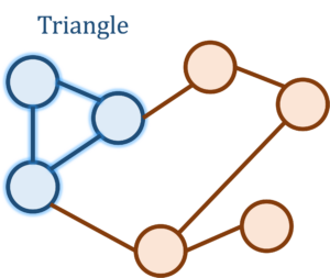
Let’s begin our discussion of concentration inequalities by means of an extended example. Consider the following question: How many triangles are there in the Facebook network? That is, how many trios of people are there who are all mutual friends? While seemingly silly at first sight, this is actually a natural and meaningful question about the structure of the Facebook social network and is related to similar questions such as “How likely are two friends of a person to also be friends with each other?”

If there are $n$ people on the Facebook graph, then the natural algorithm of iterating over all ${n \choose 3} \approx n^3/6$ triplets and checking whether they form a triangle is far too computationally costly for the billions of Facebook accounts. Somehow, we want to do much faster than this, and to achieve this speed we would be willing to settle for an estimate of the triangle count up to some error.

There are many approaches to this problem, but let’s describe a particularly surprising algorithm. Let $A$ be an $n\times n$ matrix where the $ij$ th entry of $A$ is $1$ if users $i$ and $j$ are friends and $0$ otherwise¹; this matrix is called the adjacency matrix of the Facebook graph. A fact from graph theory is that the $ij$ th entry of the cube $A^3$ of the matrix $A$ counts the number of paths from user $i$ to user $j$ of length three.² In particular, the $ii$ th entry of $A^3$ denotes the number of paths from $i$ to itself of length $3$ , which is twice the number of triangles incident on $i$ . (The paths $i\to j \to k \to i$ and $i\to k \to j\to i$ are both counted as paths of length 3 for a triangle consisting of $i$ , $j$ , and $k$ .) Therefore, the trace of $A^3$ , equal to the sum of its diagonal entries, is six times the number of triangles: The $ii$ th entry of $A^3$ is twice the number of triangles incident on $i$ and each triangle $(i,j,k)$ is counted thrice in the $ii$ th, $jj$ th, and $kk$ th entries of $A^3$ . In summary, we have

$\begin{equation*} \mbox{\# triangles} = \frac{1}{6} \operatorname{tr} A^3. \end{equation*}$

Therefore, the triangle counting problem is equivalent to computing the trace of $A^3$ . Unfortunately, the problem of computing $A^3$ is, in general, very computationally costly. Therefore, we seek ways of estimating the trace of a matrix without forming it.

Randomized Trace Estimation

Motivated by the triangle counting problem from the previous section, we consider the problem of estimating the trace of a matrix $M$ . We assume that we only have access to the matrix $M$ through matrix–vector products; that is, we can efficiently compute $Mx$ for a vector $x$ . For instance, in the previous example, the Facebook graph has many fewer friend relations (edges) $m$ than the maximum possible amount of ${n\choose 2} \approx n^2/2$ . Therefore, the matrix $A$ is sparse; in particular, matrix–vector multiplications with $A$ can be computed in around $m$ operations. To compute matrix–vector products $Mx$ with $M = A^3$ , we simply compute matrix–vector products with $A$ three times, $x \mapsto Ax \mapsto A(Ax) \mapsto A(A(Ax)) = A^3x$ .

Here’s a very nifty idea to estimate the trace of $M$ using only matrix–vector products, originally due to Didier A. Girard and Michael F. Hutchinson. Choose $x$ to be a random vector whose entries are independent $\pm 1$ -values, where each value $+1$ and $-1$ occurs with equal $1/2$ probability. Then if one forms the expression $x^\top M x = \sum_{i,j=1}^n M_{ij} x_i x_j$ . Since the entries of $x_i$ and $x_j$ are independent, the expectation of $x_ix_j$ is $0$ for $i\ne j$ and $1$ for $i = j$ . Consequently, by linearity of expectation, the expected value of $x^\top M x$ is

$\begin{equation*} \mathbb{E} \, x^\top M x = \sum_{i,j=1}^n M_{ij} \mathbb{E} [x_ix_j] = \sum_{i = 1}^n M_{ii} = \operatorname{tr}(M). \end{equation*}$

The average value of $x^\top M x$ is equal to the trace of $M$ ! In the language of statistics, we might say that $x^\top M x$ is an unbiased estimator for $\operatorname{tr}(M)$ . Thus, the efficiently computable quantity $x^\top M x$ can serve as a (crude) estimate for $\operatorname{tr}(M)$ .

While the expectation of $x^\top Mx$ equals $\operatorname{tr}(M)$ , any random realization of $x^\top M x$ can deviate from $\operatorname{tr}(M)$ by a non-neligible amount. Thus, to reduce the variability of the estimator $x^\top M x$ , it is appropriate to take an average of multiple copies of this random estimate. Specifically, we draw $k$ random vectors with independent random $\pm 1$ entries $x_1,\ldots,x_k$ and compute the averaged trace estimator

(1) $\begin{equation*} T_k := \frac{1}{k} \sum_{j=1}^k x_j^\top M x_j^{\vphantom{\top}}. \end{equation*}$

The $k$ -sample trace estimator $T_k$ remains an unbiased estimator for $\operatorname{tr}(M)$ , $\mathbb{E}\, T_k = \operatorname{tr}(M)$ , but with reduced variability. Quantitatively, the variance of $T_k$ is $k$ times smaller than the single-sample estimator $x^\top M x$ :

(2) $\begin{equation*} \operatorname{Var}(T_k) = \frac{1}{k} \operatorname{Var}(x^\top M x). \end{equation*}$

The Girard–Hutchinson trace estimator gives a natural way of estimating the trace of the matrix $M$ , a task which might otherwise be hard without randomness.³ For the trace estimator to be a useful tool, an important question remains: How many samples $k$ are needed to compute $\operatorname{tr}(M)$ to a given accuracy? Concentration inequalities answer questions of this nature.

Concentration Inequalities

A concentration inequality provides a bound on the probability a random quantity is significantly larger or smaller than its typical value. Concentration inequalities are useful because they allow us to prove statements like “With at least 99% probability, the randomized trace estimator with 100 samples produces an approximation of the trace which is accurate up to error no larger than $0.001$ .” In other words, concentration inequalities can provide quantitative estimates of the likely size of the error when a randomized algorithm is executed.

In this section, we shall introduce a handful of useful concentration inequalities, which we will apply to the randomized trace estimator in the next section. We’ll then discuss how these and other concentration inequalities can be derived in the following section.

Markov’s Inequality

Markov’s inequality is the most fundamental concentration inequality. When used directly, it is a blunt instrument, requiring little insight to use and producing a crude but sometimes useful estimate. However, as we shall see later, all of the sophisticated concentration inequalities that will follow in this post can be derived from a careful use of Markov’s inequality.

The wide utility of Markov’s inequality is a consequence of the minimal assumptions needed for its use. Let $X$ be any nonnegative random variable. Markov’s inequality states that the probability that $X$ exceeds a level $t > 0$ is bounded by the expected value of $X$ over $t$ . In equations, we have

(3) $\begin{equation*} \mathbb{P} \left\{ X \ge t \right\} \le \frac{\mathbb{E} \, X}{t}. \end{equation*}$

We stress the fact that we make no assumptions on how the random quantity $X$ is generated other than that $X$ is nonnegative.

As a short example of Markov’s inequality, suppose we have a randomized algorithm which takes one second on average to run. Markov’s inequality then shows that the probability the algorithm takes more than 100 seconds to run is at most $1/100 = 1\%$ . This small example shows both the power and the limitation of Markov’s inequality. On the negative side, our analysis suggests that we might have to wait as much as 100 times the average runtime for the algorithm to complete running with 99% probability; this large huge multiple of 100 seems quite pessimistic. On the other hand, we needed no information whatsoever about how the algorithm works to do this analysis. In general, Markov’s inequality cannot be improved without more assumptions on the random variable $X$ .⁴

Chebyshev’s Inequality and Averages

The variance of a random variable describes the expected size of a random variable’s deviation from its expected value. As such, we would expect that the variance should provide a bound on the probability a random variable is far from its expectation. This intuition indeed is correct and is manifested by Chebyshev’s inequality. Let $X$ be a random variable (with finite expected value) and $t > 0$ . Chebyshev’s inequality states that the probability that $X$ deviates from its expected value by more than $t$ is at most $\operatorname{Var}(X)/t^2$ :

(4) $\begin{equation*} \mathbb{P} \left\{ \left| X - \mathbb{E} \, X \right| \ge t \right\} \le \frac{\operatorname{Var}(X)}{t^2}. \end{equation*}$

Chebyshev’s inequality is frequently applied to sums or averages of independent random quantities. Suppose $X_1,\ldots,X_n$ are independent and identically distributed random variables with mean $\mu$ and variance $\sigma^2$ and let $\overline{X}$ denote the average

$\begin{equation*} \overline{X} = \frac{X_1 + \cdots + X_n}{n}. \end{equation*}$

Since the random variables $X_1,\ldots,X_n$ are independent,⁵ the properties of variance entail that

$\begin{equation*} \operatorname{Var}(\overline{X}) = \operatorname{Var}\left( \frac{1}{n} X_1 + \cdots + \frac{1}{n} X_n \right) = \frac{1}{n^2} \operatorname{Var}(X_1) + \cdots + \frac{1}{n^2} \operatorname{Var}(X_n) = \frac{\sigma^2}{n}, \end{equation*}$

where we use the fact that $\operatorname{Var}(X_1) = \cdots = \operatorname{Var}(X_n) = \sigma^2$ . Therefore, by Chebyshev’s inequality,

(5) $\begin{equation*} \mathbb{P} \left\{ \left| \overline{X} - \mu \right| \ge t \right\} \le \frac{\sigma^2}{nt^2}. \end{equation*}$

Suppose we want to estimate the mean $\mu$ by $\overline{X}$ up to error $\epsilon$ and are willing to tolerate a failure probability of $\delta$ . Then setting the right-hand side of (5) to $\delta$ , Chebyshev’s inequality suggests that we need at most

(6) $\begin{equation*} n = \sigma^2\cdot \frac{1/\delta}{\epsilon^2} \end{equation*}$

samples to achieve this goal.

Exponential Concentration: Hoeffding and Bernstein

How happy should we be with the result (6) of applying Chebyshev’s inequality the average $\overline{X}$ ? The central limit theorem suggests that $\overline{X}$ should be approximately normally distributed with mean $\mu$ and variance $\sigma^2/n$ . Normal random variables have an exponentially small probability of being more than a few standard deviations above their mean, so it is natural to expect this should be true of $\overline{X}$ as well. Specifically, we expect a bound roughly like

(7) $\begin{equation*} \mathbb{P} \left\{ \left| \overline{X} - \mu \right| \ge t \right\} \stackrel{?}{\lessapprox} \exp\left(-\frac{nt^2}{2\sigma^2}\right). \end{equation*}$

Unfortunately, we don’t have a general result quite this nice without additional assumptions, but there are a diverse array of exponential concentration inequalities available which are quite useful in analyzing sums (or averages) of independent random variables that appear in applications.

Hoeffding’s inequality is one such bound. Let $X_1,\ldots,X_n$ be independent (but not necessarily identically distributed) random variables and consider the average $\overline{X} = (X_1 + \cdots + X_n)/n$ . Hoeffding’s inequality makes the assumption that the summands are bounded, say within an interval $[a,b]$ .⁶ Hoeffding’s inequality then states that

(8) $\begin{equation*} \mathbb{P}\left\{ \left|\overline{X} - \mathbb{E} \, \overline{X}\right| \ge t \right\} \le 2 \exp\left( -\frac{2nt^2}{(b-a)^2} \right). \end{equation*}$

Hoeffding’s inequality is quite similar to the ideal concentration result (7) except with the variance $\sigma^2 = n\operatorname{Var}(\overline{X})$ replaced by the potentially much larger quantity⁷ $(b-a)^2/4$ .

Bernstein’s inequality fixes this deficit in Hoeffding’s inequality at a small cost. Now, instead of assuming $X_1,\ldots,X_n$ are bounded within the interval $[a,b]$ , we make the alternate boundedness assumption $|X_i - \mathbb{E}\, X_i| \le B$ for every $1\le i\le n$ . We continue to denote $\sigma^2 = n\operatorname{Var}(\overline{X})$ so that if $X_1,\ldots,X_n$ are identically distributed, $\sigma^2$ denotes the variance of each of $X_1,\ldots,X_n$ . Bernstein’s inequality states that

(9) $\begin{equation*} \mathbb{P}\left\{ \left|\overline{X} - \mathbb{E} \, \overline{X}\right| \ge t \right\} \le 2 \exp\left( -\frac{nt^2/2}{\sigma^2 + Bt/3} \right). \end{equation*}$

For small values of $t$ , Bernstein’s inequality yields exactly the kind of concentration that we would hope for from our central limit theorem heuristic (7). However, for large values of $t$ , we have

$\begin{equation*} \mathbb{P}\left\{ \left|\overline{X} - \mathbb{E} \, \overline{X}\right| \ge t \right\} \stackrel{\mbox{large $t$}}{\lessapprox} 2 \exp\left( -\frac{3nt}{2B} \right), \end{equation*}$

which is exponentially small in $t$ rather than $t^2$ . We conclude that Bernstein’s inequality provides sharper bounds then Hoeffding’s inequality for smaller values of $t$ but weaker bounds for larger values of $t$ .

Chebyshev vs. Hoeffding vs. Bernstein

Let’s return to the situation where we seek to estimate the mean $\mu$ of independent and identically distributed random variables $X_1,\ldots,X_n$ each with variance $\sigma^2$ by using the averaged value $\overline{X} = (X_1 + \cdots + X_n)/n$ . Our goal is to bound how many samples $n$ we need to estimate $\mu$ up to error $\epsilon$ , $| \overline{X} - \mu | \le \epsilon$ , except with failure probability at most $\delta$ . Using Chebyshev’s inequality, we showed that (see (7))

$\begin{equation*} n \ge \sigma^2\cdot \frac{1/\delta}{\epsilon^2} \mbox{ suffices}. \end{equation*}$

Now, let’s try using Hoeffding’s inequality. Suppose that $X_1,\ldots,X_n$ are bounded in the interval $[a,b]$ . Then Hoeffding’s inequality (8) shows that

$\begin{equation*} n \ge \frac{(b-a)^2}{4}\cdot \frac{2\log(2/\delta)}{\epsilon^2} \mbox{ suffices}. \end{equation*}$

Bernstein’s inequality states that if $X_1,\ldots,X_n$ lie in the interval $[\mu-B,\mu+B]$ for every $1\le i \le n$ , then

(10) $\begin{equation*} n \ge \sigma^2 \cdot \frac{2\log(2/\delta)}{\epsilon^2} + B\cdot \frac{2/3\cdot\log(2/\delta)}{\epsilon} \mbox{ suffices}. \end{equation*}$

Hoeffding’s and Bernstein’s inequality show that we need $n$ roughly proportional to $\tfrac{\log(1/\delta)}{\epsilon^2}$ samples are needed rather than proportional to $\tfrac{1/\delta}{\epsilon^2}$ . The fact that we need proportional to $1/\epsilon^2$ samples to achieve error $\epsilon$ is a consequence of the central limit theorem and is something we would not be able to improve with any concentration inequality. What exponential concentration inequalities allow us to do is to improve the dependence on the failure probability from proportional to $1/\delta$ to $\log(1/\delta)$ , which is a huge improvement.

Hoeffding’s and Bernstein’s inequalities both have a small drawback. For Hoeffding’s inequality, the constant of proportionality is $(b-a)^2/4$ rather than the true variance $\sigma^2$ of the summands. Bernstein’s inequality gives us the “correct” constant of proportionality $\sigma^2$ but adds a second term proportional to $\tfrac{\log(1/\delta)}{\epsilon}$ ; for small values of $\epsilon$ , this term is dominated by the term proportional to $\tfrac{\log(1/\delta)}{\epsilon^2}$ but the second term can be relevant for larger values of $\epsilon$ .

There are a panoply of additional concentration inequalities than the few we’ve mentioned. We give a selected overview in the following optional section.

Other Concentration Inequalities

There are a handful more exponential concentration inequalities for sums of independent random variables such as Chernoff’s inequality (very useful for somes of bounded, positive random variables) and Bennett’s inequality. There are also generalizations of Hoeffding’s, Chernoff’s, and Bernstein’s inequalities for unbounded random variables with subgaussian and subexponential tail decay; these results are documented in Chapter 2 of Roman Vershynin’s excellent book High-Dimensional Probability.

One can also generalize concentration inequalities to so-called martingale sequences, which can be very useful for analyzing adaptive algorithms. These inequalities can often have the advantage of bounding the probability that a martingale sequence ever deviates by some amount from its applications; these results are called maximal inequalities. Maximal analogs of Markov’s and Chebyshev’s inequalities are given by Ville’s inequality and Doob’s inequality. Exponential concentration inequalities include the Hoeffding–Azuma inequality and Freedman’s inequality.

Finally, we note that there are many concentration inequalities for functions of independent random variables other than sums, usually under the assumption that the function is Lipschitz continuous. There are exponential concentration inequalities for functions with “bounded differences”, functions of Gaussian random variables, and convex functions of bounded random variables. References for these results include Chapters 3 and 4 of the lecture notes Probability in High Dimension by Ramon van Handel and the comprehensive monograph Concentration Inequalities by Stéphane Boucheron, Gábor Lugosi, and Pascal Massart.

Analysis of Randomized Trace Estimator

Let us apply some of the concentration inequalities we introduced in last section to analyze the randomized trace estimator. Our goal is not to provide the best possible analysis of the trace estimator,⁸ but to demonstrate how the general concentration inequalities we’ve developed can be useful “out of the box” in analyzing algorithms.

In order to apply Chebyshev’s and Berstein’s inequalities, we shall need to compute or bound the variance of the single-sample trace estimtor $x^\top Mx$ , where $x$ is a random vector of independent $\pm 1$ -values. This is a straightforward task using properties of the variance:

$\begin{equation*} \operatorname{Var}(x^\top M x) = \operatorname{Var}\left( 2\sum_{i< j} M_{ij} x_i x_j \right) = 4\sum_{i\ne j, \: k\ne \ell} M_{ij} M_{k\ell} \operatorname{Cov}(x_ix_j,x_kx_\ell) = 4\sum_{i < j} M_{ij}^2 \le 2 \|M\|_{\rm F}^2 \end{equation*}$

Here, $\operatorname{Cov}$ is the covariance and $\|\cdot\|_{\rm F}$ is the matrix Frobenius norm. Chebyshev’s inequality (5), then gives

$\begin{equation*} \mathbb{P} \left\{ \left|T_k - \operatorname{tr}(M)\right| \ge t \right\} \le \frac{2\|M\|_{\rm F}^2}{kt^2}. \end{equation*}$

Let’s now try applying an exponential concentration inequality. We shall use Bernstein’s inequality, for which we need to bound $|x^\top M x - \operatorname{tr}(M)|$ . By the Courant–Fischer minimax principle, we know that $x^\top M x$ is between $\lambda_{\rm min}(M) \cdot \|x\|^2$ and $\lambda_{\rm max} (M)\cdot\|x\|^2$ where $\lambda_{\rm min}(M)$ and $\lambda_{\rm max}(M)$ are the smallest and largest eigenvalues of $M$ and $\|x\|$ is the Euclidean norm of the vector $x$ . Since all the entries of $x$ have absolute value $1$ , we have $\|x\| = \sqrt{n}$ so $x^\top M x$ is between $n\lambda_{\rm min}(M)$ and $n\lambda_{\rm max}(M)$ . Since the trace equals the sum of the eigenvalues of $M$ , $\operatorname{tr}(M)$ is also between $n\lambda_{\rm min}(M)$ and $n\lambda_{\rm max}(M)$ . Therefore,

$\begin{equation*} \left| x^\top M x - \operatorname{tr}(M) \right| \le n \left( \lambda_{\rm max}(M) - \lambda_{\rm min}(M)\right) \le 2 n \|M\|, \end{equation*}$

where $\|\cdot\|$ denotes the matrix spectral norm. Therefore, by Bernstein’s inequality (9), we have

$\begin{equation*} \mathbb{P} \left\{ \left| T_k - \operatorname{tr}(M) \right| \ge t \right\} \le 2\exp\left( -\frac{kt^2}{4\|M\|_{\rm F}^2 + 4/3\cdot tn\|M\|} \right). \end{equation*}$

In particular, (10) shows that

$\begin{equation*} k \ge \left( \frac{4\|M\|_{\rm F}^2}{\epsilon^2} + \frac{4n\|M\|}{3\epsilon} \right) \log \left(\frac{2}{\delta} \right) \end{equation*}$

samples suffice to estimate $\operatorname{tr}(M)$ to error $\epsilon$ with failure probability at most $\delta$ . Concentration inequalities easily furnish estimates for the number of samples needed for the randomized trace estimator.

We have now accomplished our main goal of using concentration inequalities to analyze the randomized trace estimator, which in turn can be used to solve the triangle counting problem. We leave some additional comments on trace estimation and triangle counting in the following bonus section.

More on Trace Estimation and Triangle Counting

To really complete the analysis of the trace estimator in an application (e.g., triangle counting), we would need to obtain bounds on $\|M\|_{\rm F}$ and $\|M\|$ . Since we often don’t know good bounds for $\|M\|_{\rm F}$ and $\|M \|$ , one should really use the trace estimator together with an a posteriori error estimates for the trace estimator, which provide a confidence interval for the trace rather than a point estimate; see sections 4.5 and 4.6 in this survey for details.

One can improve on the Girard–Hutchinson trace estimator by using a variance reduction technique. One such variance reduction technique was recently proposed under the name Hutch++, extending ideas by Arjun Singh Gambhir, Andreas Stathopoulos, and Kostas Orginos and Lin Lin. In effect, these techniques improve the number of samples $k$ needed to estimate the trace of a positive semidefinite matrix $A$ to relative error $\epsilon$ to proportional to $1/\epsilon$ down from $1/\epsilon^2$ .

Several algorithms have been proposed for triangle counting, many of them randomized. This survey gives a comparison of different methods for the triangle counting problem, and also describes more motivation and applications for the problem.

Deriving Concentration Inequalities

Having introduced concentration inequalities and applied them to the randomized trace estimator, we now turn to the question of how to derive concentration inequalities. Learning how to derive concentration inequalities is more than a matter of mathematical completeness since one can often obtain better results by “hand-crafting” a concentration inequality for a particular application rather than applying a known concentration inequality. (Though standard concentration inequalities like Hoeffding’s and Bernstein’s often give perfectly adequate answers with much less work.)

Markov’s Inequality

At the most fundamental level, concentration inequalities require us to bound a probability by an expectation. In achieving this goal, we shall make a simple observation: The probability that $X$ is larger than or equal to $t$ is the expectation of a random variable $\mathbf{1}_{[t,\infty)}(X)$ .⁹ Here, $\mathbf{1}_{[t,\infty)}(\cdot)$ is an indicator function which outputs one if its input is larger than or equal to $t$ and zero otherwise.

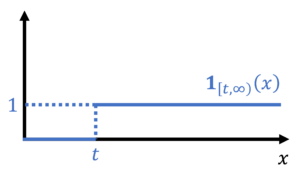
As promised, the probability $X$ is larger than $t$ is the expectation of $\mathbf{1}_{[t,\infty)}(X)$ :

(11) $\begin{equation*} \mathbb{P}\{X \ge t \} = \mathbb{E}[\mathbf{1}_{[t,\infty)}(X)]. \end{equation*}$

We can now obtain bounds on the probability that $X\ge t$ by bounding its corresponding indicator function. In particular, we have the inequality

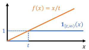
(12) $\begin{equation*} \mathbf{1}_{[t,\infty)}(x) \le \frac{x}{t} \mbox{ for every } x\ge 0. \end{equation*}$

Since $X$ is nonnegative, combining equations (11) and (12) gives Markov’s inequality:

$\begin{equation*} \mathbb{P}\{ X \ge t \} = \mathbb{E}[\mathbf{1}_{[t,\infty)}(X)] \le \mathbb{E} \left[ \frac{X}{t} \right] = \frac{\mathbb{E} X}{t}. \end{equation*}$

Chebyshev’s Inequality

Before we get to Chebyshev’s inequality proper, let’s think about how we can push Markov’s inequality further. Suppose we find a bound on the indicator function $\mathbf{1}_{[t,\infty)}(\cdot)$ of the form

(13) $\begin{equation*} \mathbf{1}_{[t,\infty)}(x) \le f(x) \mbox{ for all } x\ge 0. \end{equation*}$

A bound of this form immediately to bounds on $\mathbb{P} \{X \ge t\}$ by (11). To obtain sharp and useful bounds on $\mathbb{P}\{X\ge t\}$ we seek bounding functions $f(\cdot)$ in (13) with three properties:

For $x\in[0, t)$ , $f(x)$ should be close to zero,
For $x\in [t,\infty)$ , $f(x)$ should be close to one, and
We need $\mathbb{E} \, f(X)$ to be easily computable or boundable.

These three objectives are in tension with each other. To meet criterion 3, we must restrict our attention to pedestrian functions $f(\cdot)$ such as powers $f(x) = (x/t)^\theta$ or exponentials $f(x) = \exp(\theta (x-t))$ for which we have hopes of computing or bounding $\mathbb{E} \, f(X)$ for random variables $X$ we encounter in practical applications. But these candidate functions $f(\cdot)$ have the undesirable property that making the function smaller on $[0, t)$ (by increasing $\theta$ ) to meet point 1 makes the function larger on $(t,\infty)$ , detracting from our ability to achieve point 2. We shall eventually come up with a best-possible resolution to this dilemma by formulating this as an optimization problem to determine the best choice of the parameter $\theta > 0$ to obtain the best possible candidate function of the given form.

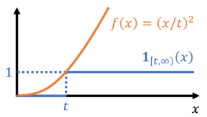
Before we get ahead of ourselves, let us use a specific choice for $f(\cdot)$ different than we used to prove Markov’s inequality. We readily verify that $f(x) = (x/t)^2$ satisfies the bound (13), and thus by (12),

(14) $\begin{equation*} \mathbb{P} \{ X \ge t \} \le \mathbb{E} \left( \frac{X}{t} \right)^2 = \frac{\mathbb{E} X^2}{t^2}. \end{equation*}$

This inequality holds for any nonnegative random variable $X$ . In particular, now consider a random variable $X$ which we do not assume to be nonnegative. Then $X$ ‘s deviation from its expectation, $|X-\mathbb{E} X|$ , is a nonnegative random variable. Thus applying (14) gives

$\begin{equation*}\mathbb{P} \{ |X - \mathbb{E} X| \ge t \} \le \frac{\mathbb{E} | X - \mathbb{E} X|^2}{t^2} = \frac{\operatorname{Var}(X)}{t^2}. \end{equation*}$

We have derived Chebyshev’s inequality! Alternatively, one can derive Chebyshev’s inequality by noting that $|X-\mathbb{E} X| \ge t$ if, and only if, $|X-\mathbb{E} X|^2 \ge t^2$ . Therefore, by Markov’s inequality,

$\begin{equation*} \mathbb{P} \{ |X - \mathbb{E} X| \ge t \} = \mathbb{P} \{ |X - \mathbb{E} X|^2 \ge t^2 \} \le \frac{\mathbb{E} | X - \mathbb{E} X|^2}{t^2} = \frac{\operatorname{Var}(X)}{t^2}. \end{equation*}$

The Laplace Transform Method

We shall now realize the plan outlined earlier where we shall choose an optimal bounding function $f(\cdot)$ from the family of exponential functions $f(x) = \exp(\theta(x-t))$ , where $\theta > 0$ is a parameter which we shall optimize over. This method shall allow us to derive exponential concentration inequalities like Hoeffding’s and Bernstein’s. Note that the exponential function $f(x) = \exp(\theta(x-t))$ bounds the indicator function $\mathbf{1}_{[t,\infty)}(\cdot)$ for all real numbers $x$ , so we shall no longer require the random variable $X$ to be nonnegative. Therefore, by (11),

(15) $\begin{equation*} \mathbb{P} \{ X \ge t \} \le \mathbb{E} \exp\left(\theta (X-t)\right) = \exp(-\theta t) \,\mathbb{E} \exp(\theta X) = \exp\left(-\theta t + \log \mathbb{E} \exp(\theta X) \right). \end{equation*}$

The functions

$\begin{equation*} m_X(\theta) = \mathbb{E} \exp(\theta X), \quad \xi_X(\theta) = \log \mathbb{E} \exp(\theta X) = \log m_X(\theta) \end{equation*}$

are known as the moment generating function and cumulant generating function of the random variable $X$ .¹⁰ With these notations, (15) can be written

(16) $\begin{equation*} \mathbb{P} \{ X \ge t \} \le\exp(-\theta t) m_X(\theta) = \exp\left(-\theta t + \xi_X(\theta) \right). \end{equation*}$

The moment generating function coincides with the Laplace transform $\mathbb{E} \exp(-\theta X) = m_X(-\theta)$ up to the sign of the parameter $\theta$ , so one name for this approach to deriving concentration inequalities is the Laplace transform method. (This method is also known as the Cramér–Chernoff method.)

The cumulant generating function has an important property for deriving concentration inequalities for sums or averages of independent random variables: If $X_1,\ldots,X_n$ are independent random variables, than the cumulant generating function is additive:¹¹

(17) $\begin{equation*} \xi_{X_1 + \cdots + X_n}(\theta) = \xi_{X_1}(\theta) + \cdots + \xi_{X_n}(\theta). \end{equation*}$

Proving Hoeffding’s Inequality

For us to use the Laplace transform method, we need to either compute or bound the cumulant generating function. Since we are interested in general concentration inequalities which hold under minimal assumptions such as boundedness, we opt for the latter. Suppose $a\le X \le b$ and consider the cumulant generating function of $Y:=X-\mathbb{E}X$ . Then one can show the cumulant generating function bound¹²

(18) $\begin{equation*} \xi_Y(\theta) \le \frac{1}{8} \theta^2(b-a)^2. \end{equation*}$

Using the additivity of the cumulant generating function (17), we obtain the bound

$\begin{equation*} \xi_{\overline{X} - \mathbb{E} \overline{X}}(\theta) = \xi_{X_1/n- \mathbb{E}X_1/n}(\theta) + \cdots + \xi_{X_n/n- \mathbb{E}X_n/n}(\theta) \le \frac{1}{n} \cdot \frac{1}{8} \theta^2(b-a)^2. \end{equation*}$

Plugging this into the probability bound (16), we obtain the concentration bound

(19) $\begin{equation*} \mathbb{P} \left\{ \overline{X} - \mathbb{E} \overline{X} \ge t \right\} \le \exp \left( - \theta t +\frac{1}{n} \cdot \frac{1}{8} \theta^2(b-a)^2 \right). \end{equation*}$

We want to obtain the smallest possible upper bound on this probability, so it behooves us to pick the value of $\theta > 0$ which makes the right-hand side of this inequality as small as possible. To do this, we differentiate the contents of the exponential and set to zero, obtaining

$\begin{equation*} \frac{\mathrm{d}}{\mathrm{d} \theta} \left( - \theta t + \frac{1}{n} \cdot \frac{1}{8} \theta^2(b-a)^2\right) = - t + \frac{1}{n} \cdot \frac{1}{4} (b-a)^2 \theta = 0\implies \theta = \frac{4nt}{(b-a)^2} \end{equation*}$

Plugging this value for $\theta$ into the bound (19) gives A bound for $\overline{X}$ being larger than $\mathbb{E}\overline{X} + t$ :

(20) $\begin{equation*} \mathbb{P} \left\{ \overline{X} - \mathbb{E} \overline{X} \ge t \right\} \le \exp \left( - \frac{2nt^2}{(b-a)^2} \right). \end{equation*}$

To get the bound on $\overline{X}$ being smaller than $\mathbb{E}\overline{X} - t$ , we can apply a small trick. If we apply (20) to the summands $-X_1,-X_2,\ldots,-X_n$ instead of $X_1,\ldots,X_n$ , we obtain the bounds

(21) $\begin{equation*} \mathbb{P} \left\{ \overline{X} - \mathbb{E} \overline{X} \le -t \right\} \le \exp \left( - \frac{2nt^2}{(b-a)^2} \right). \end{equation*}$

We can now combine the upper tail bound (19) with the lower tail bound (21) to obtain a “symmetric” bound on the probability that $|\overline{X} - \mathbb{E}\overline{X}| \ge t$ . The means of doing often this goes by the fancy name union bound, but the idea is very simple:

$\begin{equation*} \mathbb{P}(\textnormal{A happens or B happens} )\le \mathbb{P}(\textnormal{A happens}) + \mathbb{P}(\textnormal{B happens}). \end{equation*}$

Thus, applying this union bound idea with the upper and lower tail bounds (20) and (21), we obtain Hoeffding’s inequality, exactly as it appeared above as (8):

$\begin{align*} \mathbb{P}\left\{ |\overline{X} - \mathbb{E}\overline{X}| \ge t \right\} &= \mathbb{P}\left\{ \overline{X} - \mathbb{E}\overline{X} \ge t \textnormal{ or } \overline{X} - \mathbb{E}\overline{X} \le -t \right\}\\ &\le \mathbb{P} \left\{ \overline{X} - \mathbb{E} \overline{X} \ge t \right\} + \mathbb{P} \left\{ \overline{X} - \mathbb{E} \overline{X} \le -t \right\}\\ &\le 2\exp \left( - \frac{2nt^2}{(b-a)^2} \right). \end{align*}$

Voilà! Hoeffding’s inequality has been proven! Bernstein’s inequality is proven essentially the same way except that, instead of (17), we have the cumulant generating function bound

$\begin{equation*} \xi_Y(\theta) = \frac{(\theta^2/2)\Var(Y)}{1-|\theta|/3} \end{equation*}$

for a random variable $Y$ with mean zero and satisfying the bound $|Y| \le B$ .

Upshot: Randomness can be a very effective tool for solving computational problems, even those which seemingly no connection to probability like triangle counting. Concentration inequalities are a powerful tool for assessing how many samples are needed for an algorithm based on random sampling to work. Some of the most useful concentration inequalities are exponential concentration inequalities like Hoeffding and Bernstein, which show that an average of bounded random quantities are close to their average except with exponentially small probability.

Big Ideas in Applied Math: Concentration Inequalities

Triangle Counting

Randomized Trace Estimation

Concentration Inequalities

Markov’s Inequality

Chebyshev’s Inequality and Averages

Exponential Concentration: Hoeffding and Bernstein

Chebyshev vs. Hoeffding vs. Bernstein

Analysis of Randomized Trace Estimator

Deriving Concentration Inequalities

Markov’s Inequality

Chebyshev’s Inequality

The Laplace Transform Method

Proving Hoeffding’s Inequality

3 thoughts on “Big Ideas in Applied Math: Concentration Inequalities”

Leave a Reply Cancel reply