Markov Musings 4: Should You Be Lazy?

This post is part of a series, Markov Musings, about the mathematical analysis of Markov chains. See here for the first post in the series.

In the previous post, we proved the following convergence results for a reversible Markov chain

$\chi^2\left(\rho^{(n)} \, \middle|\middle| \, \pi\right) \le \left( \max \{ \lambda_2, -\lambda_n \} \right)^{2n} \chi^2\left(\rho^{(0)} \, \middle|\middle| \, \pi\right).$

Here, $\rho^{(n)}$ denotes the distribution of the chain at time $n$ , $\pi$ denotes the stationary distribution, $\chi^2(\cdot \mid\mid \cdot)$ denotes the $\chi^2$ divergence, and $1 = \lambda_1 \ge \lambda_2 \ge \cdots \ge \lambda_m \ge -1$ denote the decreasingly ordered eigenvalues of the Markov transition matrix $P$ . To bound the rate of convergence to stationarity, we therefore must upper bound $\lambda_2$ and lower bound $\lambda_m$ .

Having to prove separate bounds for two eigenvalues is inconvenient. In the next post, we will develop tools to bound $\lambda_2$ . But what should we do about $\lambda_m?$ Fortunately, there is a trick.

It Pays to be Lazy

Call a Markov chain lazy if, at every step, the chain has at least a 50% chance of staying put. That is, $P_{ii} \ge 1/2$ for every $i$ .

Any Markov chain can be made into a lazy chain. At every step of the chain, flip a coin. If the coin is heads, perform a step of the Markov chain as normal, drawing the next step randomly according to the transition matrix $P$ . If the coin comes up tails, do nothing and stay put.

Algebraically, the lazy chain described in the previous paragraph corresponds to replacing the original transition matrix $P$ with the lazy transition matrix $P^{\rm lazy} \coloneqq (I+P)/2$ , where $I$ denotes the identity matrix. It is easy to see that the stationary distribution $\pi$ for $P$ is also a stationary distribution for $P^{\rm lazy}$ :

$\pi^\top P^{\rm lazy} = \frac{1}{2} \pi^\top P + \frac{1}{2} \pi^\top I = \frac{1}{2} \pi^\top + \frac{1}{2} \pi^\top = \pi^\top.$

The eigenvalues of the lazy transition matrix are

$\lambda_i^{\rm lazy} = \frac{1+\lambda_i}{2}.$

In particular, since all of the original eigenvalues $\lambda_i$ are $\ge -1$ , all of the eigenvalues of the lazy chain are $\ge 0$ . Thus, the smallest eigenvalue of $P^{\rm lazy}$ is always $\ge 0$ and thus, for the lazy chain, the convergence is controlled only by $\lambda_2^{\rm lazy}$ :

$\chi^2\left(\rho^{(n)} \, \middle|\middle| \, \pi\right) \le \left( \lambda_2^{\rm lazy} \right)^{2n} \chi^2\left(\rho^{(0)} \, \middle|\middle| \, \pi\right).$

Since it can be easier to establish bounds on the second eigenvalue than on both the second and last, it can be convenient—for theoretical purposes especially—to work with lazy chains, using the construction above to enforce laziness if necessary.

Should You be Lazy?

We’ve seen one theoretical argument for why it pays to use lazy Markov chains. But should we use lazy Markov chains in practice? The answer ultimately depends on how we want to use the Markov chain.

Here are two very different ways we could use a Markov chain:

One-shot sampling. Run the Markov chain once for a fixed number of steps $n$ , and use the result as an approximate sample from $\pi$ .

For this use case, it is important that the output is genuinely a sample from $\pi$ , and the possibility of large negative eigenvalues can significantly degrade the convergence. In the extreme case where $-1$ is an eigenvalue, the chain will fail to converge to stationarity at all. For this application, the lazy approach may make sense.

Averaging. Another way we can use a Markov chain is to compute the average of value of a function $f(x)$ over a random variable $x\sim\pi$ drawn from the stationary distribution:
$\expect_{x\sim \pi} [f(x)] = \sum_{i=1}^m f(i) \pi_i.$
To do this, we approximate this expectation by the time average $\hat{f}_N$ of the value of $f$ over the first $N$ values $x_0,x_1,\ldots,x_{N-1}$ of the chain
$\hat{f}_{N}\coloneqq \frac{1}{N}\sum_{n=0}^{N-1} f(x_i).$

As we shall see, this averaging process converges at an (asymptotically) slower rate for the lazy chain than the original chain. Therefore, for this application, we should typically just run the chain as-is, and not worry about making it lazy.

The Case Against Laziness

To see why being lazy hurts us for the averaging problem, we will use the Markov chain central limit theorem. As with many random averaging processes, we expect that in the limit of a large number of steps $N$ , the Markov chain average

$\hat{f}_N = \frac{1}{N}\sum_{n=0}^{N-1} f(x_i)$

will become approximately normally distributed. This is the content of the Markov chain central limit theorem (CLT):

Informal theorem (Markov chain central limit theorem). Let $x_0,x_1,x_2,\ldots$ denote the states of a Markov chain initialized in the stationary distribution $x_0\sim\pi$ . For a large number $N$ of steps, $\hat{f}_N$ is approximately normally distributed with mean $\expect_{x\sim \pi} [f(x)]$ and variance $\sigma^2/N$ where
(1) $\sigma^2 = \Var[f(x_0)] + 2\sum_{n=1}^\infty \Cov(f(x_0),f(x_n)).$

The Markov chain CLT shows that the variance of the Markov chain average $\hat{f}_N$ depends not only on the variance of $f$ in the stationary distribution, but also the covariance between $f(x_0)$ and later values $f(x_n)$ . The faster the covariance decreases, the smaller $\sigma^2$ will be and thus the smaller the error for the Markov chain average.

More formally, the Markov chain CLT is given by the following result:

Theorem (Markov chain central limit theorem). As $N\to\infty$ ,
$\frac{\hat{f}_N - \expect_{x \sim \pi} [f(x)]}{\sqrt{N}}$
converges in distribution to a normal random variable with mean zero and variance $\sigma^2$ , as defined in (1).

To compare the lazy and non-lazy chains, let’s compute the variance parameter $\sigma^2$ in the Markov chain CLT in terms of the eigenvalues of the chain. For the remainder of this post, let $f : \{1,\ldots,m\} \to \real$ be any function.

Step 1: Spectral Decomposition

Recall that, by the spectral theorem, the transition matrix $P$ has eigenvectors $\varphi_1,\varphi_2,\ldots,\varphi_m$ that are orthonormal in the $\pi$ -inner product

$\langle \varphi_i,\varphi_j \rangle = \expect_{x\sim \pi} [\varphi_i(x)\varphi_j(x)] = \begin{cases}1, & i = j, \\0, & i \ne j.\end{cases}$

As in the previous post, we think of vectors such as $\varphi_i \in \real^m$ as defining a function $\varphi_i : \{1,\ldots,m\} \to \real$ . Thus, we can expand the function $f$ using the eigenvectors

(2) $f = c_1 \varphi_1 + \cdots + c_m \varphi_m.$

The first eigenvector $\varphi_1 = \mathbf{1}$ is the vector of all ones (or, equivalently, the function that outputs $1$ for every output).

Step 2: Applying the Transition Matrix to a Function

The transition matrix $P$ is defined so that if the Markov chain has probability distribution $\sigma^\top$ at time $n$ , then the chain has distribution $\sigma^\top P$ at time $n+1$ . In other words, multiplying by $P$ on the right advances a distribution forward one step in time. This leads us to ask, what is the interpretation of multiplying a function by $P$ on the left. That is, is there an interpretation to the matrix–vector product $Pf$ ?

Indeed, there is such an interpretation: The $i$ th coordinate of $Pf$ is the expectation of $f(x_1)$ conditional on the chain starting at $x_0 = i$ :

$(Pf)(i) = \expect[f(x_1) \mid x_0 = i].$

Similarly,

(3) $(P^nf)(i) = \expect[f(x_n) \mid x_0 = i].$

There’s a straightforward proof of this fact. Let $\delta_i^\top$ denote a probability distribution which places 100% of the probability mass on the single site $i$ . The $i$ th entry of $P^n f$ is

$(P^n f)(i) = \delta_i^\top (P^n f) = (\delta_i^\top P^n) f.$

We know that $\rho^{(n)} = \delta_i^\top P^n$ is the state of the Markov chain after $n$ steps when initialized in the initial distribution $\rho^{(n)} = \delta_i$ . Thus,

$(P^n f)(i) = (\rho^{(n)})^\top f = \sum_{i=1}^m \rho^{(n)}_i f(i) = \expect[f(x_n) \mid x_0=i].$

This proves the formula (3).

Step 3: Computing the Covariance

With the help of the formula for $P^nf$ and the spectral decomposition of $f$ , we are ready to compute the covariances appearing in (1).Let $x_0 \sim \pi$ . Then

(4) $\Cov (f(x_0),f(x_n)) = \expect[f(x_0)f(x_n)] - \expect[f(x_0)]\expect[f(x_n)].$

Let’s first compute $\expect[f(x_0)]$ and $\expect[f(x_n)]$ . Since $\varphi_1 = \mathbf{1}$ is the vector/function of all ones, we have

$\expect[f(x_0)] = \expect[f(x_0) \cdot 1] = \expect[f(x_0) \varphi_1(x_0)] = \langle f, \varphi_1\rangle = c_1.$

For the last equality, we use the spectral decomposition (2) along with the orthonormality of the eigenvectors $\varphi_i$ .

Since we assume the chain is initialized in the stationary distribution $x_0 \sim \pi$ , it remains in stationarity at time $n$ , $x_n \sim \pi$ , so we have $\expect[f(x_n)] = \expect[f(x_0)] = c_1$ .

Now, let’s compute $\expect[f(x_0)f(x_n)]$ . Use the law of total expectation to write

$\begin{align*}\expect[f(x_0)f(x_n)] &= \sum_{i=1}^m \expect[f(x_0) f(x_n) \mid x_0 = i] \prob\{x_0 = i\} \\&= \sum_{i=1}^m f(i) \expect[f(x_n) \mid x_0 = i] \pi_i.\end{align*}$

Now, invoke (3) and the definition of the $\pi$ -inner product to write

$\expect[f(x_0)f(x_n)] = \sum_{i=1}^m f(i) (P^n f)(i) \pi_i = \langle f, P^n f\rangle.$

Finally, using the spectral decomposition, we obtain

$\expect[f(x_0)f(x_n)] = \left\langle \sum_{i=1}^m c_i \varphi_i,\sum_{i=1}^m c_i P^n\varphi_i \right\rangle = \left\langle \sum_{i=1}^m c_i \varphi_i,\sum_{i=1}^m c_i \lambda_i^n \varphi_i \right\rangle = \sum_{i=1}^m \lambda_i^n \, c_i^2.$

Combining this formula with our earlier observation that $\expect[f(x_0)] = \expect[f(x_n)] = c_1$ and plugging into (4), we obtain

(5) $\Cov(f(x_0),f(x_n)) = \sum_{i=1}^m \lambda_i^n \, c_i^2 - c_1^2 = \sum_{i=2}^m \lambda_i^n c_i^2.$

For the second equality, we use that the largest eigenvalue is $\lambda_1 = 1$ , so $c_1$ entirely drops out of the covariance.

Step 4: Wrapping it Up

With the formula (5) for the covariance in hand, we are ready to evaluate the $\sigma^2$ variance parameter in the Markov chain CLT. First, note that the variance is

$\Var[f(x_0)] = \Cov(f(x_0),f(x_0)) = \sum_{i=2}^m \lambda_i^0 c_i^2 = \sum_{i=2}^m c_i^2.$

Therefore, combining this formula for the variance and the formula (5) for the covariance, we obtain

$\begin{align*}\sigma^2 &= \Var[f(x_0)] + 2\sum_{n=1}^\infty \Cov(f(x_0),f(x_n)) \\&= \sum_{i=2}^m c_i^2 + 2\sum_{n=1}^\infty \sum_{i=2}^m \lambda_i^n \, c_i^2 \\&= -\sum_{i=2}^m c_i^2 + 2\sum_{i=2}^m \left(\sum_{n=0}^\infty \lambda_i^n\right)c_i^2 .\end{align*}$

Now, apply the formula for the sum of an infinite geometric series to obtain

(6) $\sigma^2 = -\sum_{i=2}^m c_i^2 + 2\sum_{i=2}^m \frac{1}{1-\lambda_i} c_i^2 = \sum_{i=2}^m \left(\frac{2}{1-\lambda_i}-1\right)c_i^2 = \sum_{i=2}^m \frac{1+\lambda_i}{1-\lambda_i} c_i^2.$

Conclusion: Laziness is (Asymptotically) Bad for Averaging

Before we get to the conclusions, let’s summarize where we are. We are seeking to use Markov chain average

$\hat{f}_N = \frac{1}{N} \sum_{i=0}^{N-1} f(x_n)$

as an approximation to the stationary mean $\expect_{x \sim \pi} [f(x)]$ . The Markov chain central limit theorem shows that, for a large number of steps $N$ , the error $\hat{f}_N - \expect_{x\sim\pi}[f(x)]$ is approximately normally distributioned with mean zero and variance $\sigma^2/N$ . So to obtain accurate estimates, we want $\sigma^2$ to be as small as possible.

After some work, we were able to derive a formula (6) for $\sigma^2$ in terms of the eigenvalues $\lambda_1,\ldots,\lambda_m$ of the transition matrix $P$ . The formula for $\sigma^2$ for the lazy chain is identical, except with each eigenvalue replaced by $(\lambda_i+1)/2$ . Thus, we have

$\begin{align*}\sigma^2_{\rm nonlazy} &= \sum_{i=2}^m \frac{1+\lambda_i}{1-\lambda_i} c_i^2, \\\sigma^2_{\rm lazy} &= \sum_{i=2}^m \frac{3+\lambda_i}{1-\lambda_i} c_i^2.\end{align*}$

From these formulas, it is clear that the lazy Markov chain has a larger $\sigma^2$ parameter and is thus less accurate than the non-lazy Markov chain, no matter what the eigenvalues are.

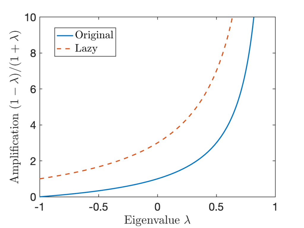
To compare the non-lazy and lazy chains in another way, consider the plot below. The blue solid line shows the amplification factor $(1-\lambda_i)/(1+\lambda_i)$ of an eigenvalue $\lambda_i$ , which represents amount by which the squared coefficient $c_i^2$ is scaled by in $\sigma^2$ . In the red-dashed line, we see the corresponding amplification factor $(1-\lambda_i^{\rm lazy})/(1+\lambda^{\rm lazy}_i)$ for the corresponding eigenvalue $\lambda^{\rm lazy}_i = (\lambda_i+1)/2$ of the lazy chain. We see that at every $\lambda$ value, the lazy chain has a higher amplification factor than the original chain.

Remember that our original motivation for using the lazy chain was to remove the possibility of slow convergence of the chain to stationarity because of negative eigenvalues. But for the averaging application, negative eigenvalues are great. The process of Markov chain averaging shrinks the influence of negative eigenvalues on $\sigma^2$ , whereas positive eigenvalues are amplified. For the averaging application, negative eigenvalues for the chain are a feature, not a bug.

Moral of the Story

Much of Markov chain theory, particularly in theoretical parts of computer science, mathematics, and machine learning, is centered around proving convergence to stationarity. Negative eigenvalues are a genuine obstruction to convergence to stationarity, and using the lazy chain in practice may be a sensible idea if one truly needs a sample from the stationary distribution in a given application.

But one-shot sampling is not the only or even the most common uses for Markov chains in computational practice. For other applications, such as averaging, the negative eigenvalues are actually a help. Using the lazy chain in practice for these problems would be a poor idea.

To me, the broader lesson in this story is that, as applied mathematicians, it can be inadvisable to become too fixated on one particular mathematical benchmark for designing and analyzing algorithms. Proving rapid convergence to stationarity with respect to the total variation distance is one nice way to analyze Markov chains. But it isn’t the only way, and chains not possessing this property because of large negative eigenvalues may actually be better in practice for some problems. Ultimately, applied mathematics should, at least in part, be guided by applications, and paying attention to how algorithms are used in practice should inform how we build and evaluate new ones.