The Hard Way to Prove Jensen’s Inequality

In this post, I want to discuss a very beautiful piece of mathematics I stumbled upon recently. As a warning, this post will be more mathematical than most, but I will still try and sand off the roughest mathematical edges. This post is adapted from a much more comprehensive post by Paata Ivanishvili. My goal is to distill the main idea to its essence, deferring the stochastic calculus until it cannot be avoided.

Jensen’s inequality is one of the most important results in probability.

Jensen’s inequality. Let $X$ be a (real) random variable and $f:\real\to\real$ a convex function such that both $\mathbb{E} X$ and $\mathbb{E} f(X)$ are defined. Then $f(\mathbb{E}X) \le \mathbb{E} [f(X)]$ .

Here is the standard proof. A convex function has supporting lines. That is, at a point $a \in \real$ , there exists a slope $m$ such that $m(x-a) + f(a) \le f(x)$ for all $x \in \real$ . Invoke this result at $a = \mathbb{E} X$ and $x = X$ and take expectations to conclude that

$\mathbb{E}[m(X - \mathbb{E}X) + f(\mathbb{E}X)] = f(\mathbb{E}X) \le \mathbb{E} [f(X)].$

In this post, I will outline a proof of Jensen’s inequality which is much longer and more complicated. Why do this? This more difficult proof illustrates an incredible powerful technique for proving inequalities, interpolation. The interpolation method can be used to prove a number of difficult and useful inequalities in probability theory and beyond. As an example, at the end of this post, we will see the Gaussian Jensen inequality, a striking generalization of Jensen’s inequality with many applications.

The idea of interpolation is as follows: Suppose I wish to prove $A_0 \le A_1$ for two numbers $A_0$ and $A_1$ . This may hard to do directly. With the interpolation method, I first construct a family of numbers $A_t$ , $0 \le t \le 1$ , such that $A_{t = 0} = A_0$ and $A_{t=1} = A_1$ and show that $(A_t : 0\le t\le 1)$ is (weakly) increasing in $t$ . This is typically accomplished by showing the derivative is nonnegative:

$\frac{d}{dt} A_t \ge 0.$

To prove Jensen’s inequality by interpolation, we shall begin with a special case. As often in probability, the simplest case is that of a Gaussian random variable.

Jensen’s inequality for a Gaussian. Let $X$ be a standard Gaussian random variable (i.e., mean-zero and variance $1$ ) and let $f:\real\to\real$ be a thrice-differentiable convex function satisfying a certain technical condition.¹ Then
$f(0) \le \mathbb{E} [f(X)].$

Note that the conclusion is exactly Jensen’s inequality, as we have assumed $X$ is mean-zero.

The difficulty with any proof by interpolation is to come up with the “right” $A_t$ . For us, the “right” answer will take the form

$A_t = \mathbb{E} [ f(X_t) ],$

where $X_0 = 0$ starts with no randomness and $X_1 = X$ is our standard Gaussian. To interpolate between these extremes, we increase the variance linearly from $0$ to $1$ . Thus, we define

$A_t = \mathbb{E} [ f(X_t)] \quad \text{where $X_t\sim\mathcal{N}(0,t)$}.$

Here, and throughout, $\mathcal{N}(0,v)$ denotes a Gaussian random variable with zero mean and variance $v$ .

Let’s compute the derivative of $A_t$ . To do this, let $\delta > 0$ denote a small parameter which we will later send to zero. For us, the key fact will be that a $\mathcal{N}(0,t+\delta)$ can be realized as a sum of independent $\mathcal{N}(0,t)$ and $\mathcal{N}(0,\delta)$ random variables. Therefore, we write

$X_{t+\delta} = X_t + \Delta \quad \text{where $\Delta \sim \mathcal{N}(0,\delta)$ is independent of $X_t$.}$

We now evaluate $f(X_t+\Delta)$ by using Taylor’s formula

(1) $f(X_t+\Delta) = f(X_t) + f'(X_t)\Delta + \frac{1}{2} f''(X_t) \Delta^2 + \frac{1}{6} f'''(\xi) \Delta^3,$

where $\xi$ lies between $X_t$ and $X_t+\Delta$ . Now, take expectations,

$\mathbb{E}[ f(X_t+\Delta)]=\mathbb{E}[f(X_t)] + \mathbb{E}[f'(X_t)\Delta] + \frac{1}{2} \mathbb{E}[f''(X_t)] \mathbb{E}[\Delta^2] + \underbrace{\frac{1}{6} \mathbb{E}[f'''(\xi) \Delta^3]}_{:=\mathrm{Rem}(\delta)}.$

The random variable $\Delta$ has mean zero and variance $\delta$ so this gives

$\mathbb{E} [f(X_t+\Delta)]=\mathbb{E}[f(X_t)] + \delta \frac{1}{2} \mathbb{E}[f''(X_t)] + \mathrm{Rem}(\delta).$

As we show below, the remainder term $\mathrm{Rem}(\delta)/\delta$ vanishes as $\delta\to 0$ . Thus, we can rearrange this expression to compute the derivative:

$\frac{d}{dt} A_t = \lim_{\delta \downarrow 0} \frac{\mathbb{E} f(X_t+\Delta)-\mathbb{E}[f(X_t)]}{\delta} = \lim_{\delta \downarrow 0} \frac{1}{2} \mathbb{E}[f''(X_t)] + \frac{\mathrm{Rem}(\delta)}{\delta} = \frac{1}{2} \mathbb{E}[f''(X_t)].$

The second derivative of a convex function is nonnegative: $f''(x) \ge 0$ for every $x$ . Therefore,

$\frac{d}{dt} A_t \ge 0 \quad \text{for all } t\in [0,1].$

Jensen’s inequality is proven! In fact, we’ve proven the stronger version of Jensen’s inequality:

$\mathbb{E} f(X) = f(0) + \frac{1}{2} \int_0^1 \mathbb{E} [f''(X_t)] \, dt.$

This strengthened version can yield improvements. For instance, if $f$ is $\beta$ -smooth

$f''(x) \le \beta \quad \text{for every } x \in \real,$

then we have

$f(0) \le \mathbb{E} f(X) \le f(0) + \frac{1}{2}\beta.$

This inequality isn’t too hard to prove directly, but it does show that we’ve obtained something more than the simple proof of Jensen’s inequality.

Analyzing the Remainder Term

Let us quickly check that the remainder term vanishes $\mathrm{Rem}(\delta)/\delta$ as $\delta \to 0$ . Let’s do this. As an exercise, you can verify that our technical regularity condition implies $\mathbb{E} |f'''(\xi)|^p < +\infty$ . Thus, by Hölder’s inequality and setting $q$ to be $p$ ‘s Hölder conjugate ( $1/p = 1/q = 1$ ), we obtain

$\frac{|\mathrm{Rem}(\delta)|}{\delta} = \frac{|\mathbb{E}[f'''(\xi) \Delta^3]|}{6\delta} \le \frac{(|\mathbb{E} |f'''(\xi)|^p)^{1/p}| (\mathbb{E} |\Delta|^{3q})^{1/q}}{6\delta}.$

One can show that $(\mathbb{E} |\Delta|^{3q})^{1/q} \le C(q) \delta^{3/2}$ where $C(q)$ is a function of $q$ alone. Therefore, $|\mathrm{Rem}(\delta)|/\delta \le \mathrm{constant} \cdot \delta^{1/2} \to 0$ as $\delta \downarrow 0$ .

What’s Really Going On Here?

In our proof, we use a family of random variables $X_t \sim \mathcal{N}(0,t)$ , defined for each $0\le t \le 1$ . Rather than treating these quantities as independent, we can think of them as a collective, comprising a random function $t \mapsto X_t$ known as a Brownian motion.

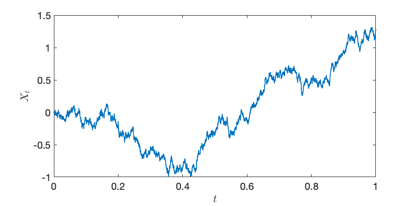
The Brownian motion is a very natural way of interpolating between a constant $\mu$ and a Gaussian with mean $\mu$ .²

There is an entire subject known as stochastic calculus which allows us to perform computations with Brownian motion and other random processes. The rules of stochastic calculus can seem bizarre at first. For a function $f$ of a real number $x$ , we often write

$df = f'(x) \, dx$

For a function $f(X_t)$ of a Brownian motion, the analog is Itô’s formula

$df = f'(X_t) \, dX_t + \frac{1}{2} f''(X_t) \, dt.$

While this might seem odd at first, this formula may seem more sensible if we compare with (1) above. The idea, very roughly, is that for an increment of the Brownian motion $dX_t$ over a time interval $dt$ , $(dX_t)^2$ is a random variable with mean $dt$ , so we cannot drop the second term in the Taylor series, even up to first order in $dt$ . Fully diving into the subtleties of stochastic calculus is far beyond the scope of this short post. Hopefully, the rest of this post, which outlines some extensions of our proof of Jensen’s inequality that require more stochastic calculus, will serve as an enticement to learn more about this beautiful subject.

Proving Jensen by Interpolation

For the rest of this post, we will be less careful with mathematical technicalities. We can use the same idea that we used to prove Jensen’s inequality for a Gaussian random variable to prove Jensen’s inequality for any random variable $Y$ :

$f(\mathbb{E}Y) \le \mathbb{E}[f(Y)].$

Here is the idea of the proof.

First, realize that we can write any random variable $Y$ as a function of a standard Gaussian random variable $X$ . Indeed, letting $F_X$ and $F_Y$ denote the cumulative distribution functions of $X$ and $Y$ , one can show that

$g(X) := \inf \{ \alpha \in \real : F_Y(\alpha) \ge F_X(X) \}$

has the same distribution as $Y$ .

Now, as before, we can interpolate between $\mathbb{E} Y$ and $Y$ using a Brownian motion. As a first, idea, we might try

$A_t \stackrel{?}{=} \mathbb{E} [f(g(X_t))].$

Unfortunately, this choice of $A_t$ does not work! Indeed, $A_0 = \mathbb{E}[f(g(0))]$ does not even equal to $\mathbb{E} [f(Y)]$ ! Instead, we must define

$A_t = \mathbb{E} [f(\mathbb{E}[g(X_1) \mid X_t])].$

We define $A_t$ using the conditional expectation of the final value $g(X_1)$ conditional on the Brownian motion $X_t$ at an earlier time $t$ . Using a bit of elbow grease and stochastic calculus, one can show that

$\frac{d}{dt} A_t \ge 0 \quad \text{for all }t\in [0,1].$

This provides a proof of Jensen’s inequality in general by the method if interpolation.

Gaussian Jensen Inequality

Now, we’ve come to the real treat, the Gaussian Jensen inequality. In the last section, we saw the sketch of a proof of Jensen’s inequality using interpolation. While it is cool that this proof is possible, we learned anything new since we can prove Jensen’s inequality in other ways. The Gaussian Jensen inequality provides an application of this technique which is hard to prove other ways. This section, in particular, is cribbing quite heavily from Paata Ivanishvili‘s excellent post on the topic.

Here’s the big question:

If $Y_1,\ldots,Y_n$ are “somewhat dependent”, for which functions does the multivariate Jensen’s inequality
( $\star$ ) $f(\mathbb{E} Y_1,\ldots,\mathbb{E}Y_n) \le \mathbb{E} [f(Y_1,\ldots,Y_n)]$
hold?

Considering extreme cases, if $Y_1,\ldots,Y_n$ are entirely dependent, then we would only expect ( $\star$ ) to hold when $f$ is convex. But if $Y_1,\ldots,Y_n$ are independent, then we can apply Jensen’s inequality to each coordinate one at a time to deduce

$\text{($\star$) holds if $f$ is convex in each coordinate, separately.}$

We would like a result which interpolates between extremes {fully dependent, fully convex} and {independent, separately convex}. The Gaussian Jensen inequality provides exactly this tool.

As in the previous section, we can generate arbitrary random variables $Y_1,\ldots,Y_n$ as functions $g(X_1),\ldots,g(X_n)$ of Gaussian random variables $X_1,\ldots,X_n$ . We will use the covariance matrix $\Sigma$ of the Gaussian random variables $X_1,\ldots,X_n$ as our measure of the dependence of the random variables $Y_1,\ldots,Y_n$ . With this preparation in place, we have the following result:

Gaussian Jensen inequality. The conclusion of Jensen’s inequality
(2) $f(\mathbb{E}g_1(X_1),\ldots,\mathbb{E}g_n(X_n)) \le \mathbb{E} [f(g(X_1),\ldots,g(X_n))]$
holds for all test functions $g_1,\ldots,g_n$ if and only if
$\Sigma \circ \nabla^2 f(x) \text{ is positive semidefinite} \quad \text{for all $x \in \real^n$}.$
Here, $\nabla^2 f(x)$ is the Hessian matrix at $x$ and $\circ$ denotes the entrywise product of matrices.

This is a beautiful result with striking consequences (see Ivanishvili‘s post). The proof is essentially the same as the proof as Jensen’s inequality by interpolation with a little additional bookkeeping.

Let us confirm this result respects our extreme cases. In the case where $X_1=\cdots=X_n$ are equal (and variance one), $\Sigma$ is a matrix of all ones and $\Sigma \circ \nabla^2 f(x) = \nabla^2 f(x)$ for all $x$ . Thus, the Gaussian Jensen inequality states that (2) holds if and only if $\nabla^2 f(x)$ is positive semidefinite for every $x$ , which occurs precisely when $f$ is convex.

Next, suppose that $X_1,\ldots,X_n$ are independent and variance one, then $\Sigma$ is the identity matrix and

$\Sigma \circ \nabla^2 f(x) = \mathrm{diag} \left( \frac{\partial^2 f}{\partial x_i^2} : i=1,\ldots,n \right).$

A diagonal matrix is positive semidefinite if and only if its entries are nonnegative. Thus, (2) holds if and only if each of $f$ ‘s diagonal second derivatives are nonnegative $\partial_{x_i}^2 f \ge 0$ : this is precisely the condition for $f$ to be separately convex in each argument.

There’s much more to be said about the Gaussian Jensen inequality, and I encourage you to read Ivanishvili‘s post to see the proof and applications. What I find so compelling about this result—so compelling that I felt the need to write this post—is how interpolation and stochastic calculus can be used to prove inequalities which don’t feel like stochastic calculus problems. The Gaussian Jensen inequality is a statement about functions of dependent Gaussian random variables; there’s nothing dynamic happening. Yet, to prove this result, we inject dynamics into the problem, viewing the two sides of our inequality as endpoints of a random process connecting them. This is a such a beautiful idea that I couldn’t help but share it.

What’s Really Going On Here?

Proving Jensen by Interpolation

Gaussian Jensen Inequality

Leave a Reply Cancel reply