Note to Self: Hanson–Wright and Trace Estimation with Random Vectors on the Sphere

November 4, 2024 by Ethan N. Epperly Leave a comment

Tyler Chen has just released an excellent monograph on the Lanczos method, one of the most powerful algorithms for extracting information from a symmetric matrix $A$ . I would definitely recommend checking it out.

One of the subjects touched on by this book is stochastic trace estimation, a topic I’ve written about several times before on this blog. In his book, Tyler uses stochastic trace estimates based on random vectors on the sphere (a great choice), and he provides a simple, but often pessimistic, mathematical analysis of this approach. To complement Tyler’s amazing book, I felt it was a good opportunity to share a sharper analysis that I came up with using a more sophisticated argument. I would not be surprised if this argument appears elsewhere in the literature, but I am not aware of a source.

Let $x,x_1,\ldots,x_m$ be random vectors in $\real^n$ drawn uniformly at random from the sphere of radius $\sqrt{n}$ ,¹ let $A$ be a real symmetric matrix, and define the quadratic form

$q \coloneqq x^\top Ax$

and the Girard–Hutchinson trace estimator

$\hat{\tr}\coloneqq \frac{1}{m}\sum_{i=1}^m x_i^\top Ax_i.$

Both $q$ and $\hat{\tr}$ are unbiased estimates for the trace of $A$ , $\expect[q] = \expect[\hat{\tr}] = \tr A$ . The goal of this post will be to bound the probability of these quantities being much smaller or larger than the trace of $A$ .

Hanson–Wright on the Sphere

Observe that $\hat{\tr}$ is an average of $m$ independent copies of the random variable $q$ . Therefore, we will begin our analysis with the quadratic form $q$ and discuss the Girard–Hutchinson estimate $\hat{\tr}$ at the end of the post.

Centering

Begin by introducing the centered matrix

$\overline{A} = A - \frac{\tr A}{n}I.$

The transformation $A\mapsto\overline{A}$ has the effect of shifting $A$ ’s eigenvalues to have mean zero. Consequently, since the trace is the sum of the eigenvalues, $\overline{A}$ has trace zero.

Now, rewrite $q$ in terms of the centered matrix $\overline{A}$ :

$q = x^\top A x = x^\top \overline{A} x + \frac{\tr A}{n} \cdot x^\top I x = x^\top \overline{A} x + \tr A.$

In the final equality, we use the fact that $x$ is on the sphere of radius $\sqrt{n}$ so that $x^\top I x = \norm{x}^2 = n$ . Rearranging, we see that the error $\overline{q}\coloneqq q-\tr A$ satisfies

$\overline{q} = q-\tr A = x^\top \overline{A}x.$

We have shown that the error $\overline{q}$ depends only on the centered matrix $\overline{A}$ rather than the original matrix $A$ . This observation is at the root of the reason that quadratic forms with vectors on the sphere have smaller tail probabilities than other distributions like the Gaussian distribution. Indeed, $\overline{A}$ is smaller than $A$ when measured using the Frobenius norm $\norm{\overline A}_{\rm F} \le \norm{A}_{\rm F}$ , and the spectral norm is never much larger $\norm{\overline{A}} \le 2\norm{A}$ . These observations will be important later.

Laplace Transform Method and Comparison to Standard Gaussian Vectors

To derive exponential concentration inequalities, we make use of the Laplace transform method. For a random variable $z$ , define the cumulant generating function (cgf)

$\xi_z(\theta) = \log (\expect [\exp(\theta z)]).$

Bounds on the cgf immediately yield bounds on the random variable taking large values, so it will behoove us to estimate this quantity for $\overline{q}$ .

To estimate the cgf of $\overline{q}$ , we will make use of a comparison between Gaussian vectors and random vectors on the sphere. Recall that a standard Gaussian vector $g$ is a vector with independent standard Gaussian entries. Standard Gaussian random vectors are spherically symmetric, meaning they can be written in the form $g = a\cdot x$ , where $x$ is a uniform random vector on the sphere and $a$ is a scaling factor.² The scaling factor $a$ is independent of $x$ and, in this case, satisfies $\expect[a^2] = 1$ .³

Using this relationship, the error $\overline{q}$ can be connected to the standard Gaussian random vector $g$ as follows

$g^\top \overline{A} g = a^2 \cdot x^\top \overline{A} x = a^2 \cdot \overline{q}.$

Intuitively, we might expect that multiplying the random error $\overline{q}$ by a scaling factor of mean one should only have the effect of increasing the variability of $\overline{q}$ and thus increasing its probability of taking large values. Based on this intuition, we might conjecture that the cgfs are related

$\xi_{\overline{q}}(\theta) \le \xi_{g^\top A g}(\theta) \quad \text{for all } \theta \in \real.$

Indeed, this conjecture is true.

Proposition (Scaling hurts). Let $z$ be a random variable and let $b$ be a random variable with expectation $1$ , independent of $z$ . Then
$\xi_{z}(\theta) \le \xi_{bz}(\theta) \quad \text{for all } \theta \in \real.$

To prove this result, let $\expect_b$ and $\expect_z$ denote expectations take over the randomness in $b$ and $z$ separately. The total expectation is $\expect[\cdot] = \expect_z[\expect_b[\cdot ]]$ . Begin with the right-hand side and invoke Jensen’s inequality over $b$ :

$\xi_{bz}(\theta) = \xi_z(\theta) = \log (\expect_z [\expect_b [\exp(\theta bz)]]) \ge \log (\expect_z [\exp(\theta \expect_b[b]z)]) = \xi_z(\theta).$

In the last line, we use the hypothesis $\expect[b] = 1$ and the definition of the cgf.

Having established this proposition, we conclude that $\xi_{\overline{q}}(\theta) \le \xi_{g^\top \overline{A} g}(\theta)$ for all $\theta$ .

Completing the Analysis

Finally, invoking a standard bound for the cgf of $g^\top \overline{A}g$ for a trace-zero matrix $\overline{A}$ , we obtain

$\xi_{\overline{q}}(\theta) \le \xi_{g^\top \overline{A} g}(\theta) \le \frac{\theta^2 \norm{\overline{A}}_{\rm F}^2}{1 - 2\theta \norm{\overline{A}}}.$

A cgf bound of this form immediately yields the following tail bound (see Boucheron, Lugosi, and Massart’s Concentration Inequalities page 29 and Exercise 2.8):

$\prob \{ x^\top A x - \tr(A) \ge t \} \le \exp \left( - \frac{t^2/2}{2 \norm{\overline{A}}_{\rm F}^2 + 2 \overline{\norm{\overline{A}}t}} \right).$

One can also control the lower tail event $x^\top A x - \tr(A) \le -t$ by instantiating this result with $-A$ . Union bounding over the upper and lower tails gives the symmetric bound

$\prob \{ |x^\top A x - \tr(A)| \ge t \} \le 2\exp \left( - \frac{t^2/2}{2 \norm{\overline{A}}_{\rm F}^2 + 2 \overline{\norm{\overline{A}}t}} \right).$

Is This Bound Good?

Tail bounds for quadratic forms such as $x^\top A x$ or $g^\top A g$ are known as Hanson–Wright inequalities. For vectors on the sphere, our bound shows the tail probabilities decay like $\exp(-O(t^2/\norm{\overline{A}_{\rm F}}^2))$ for small $t > 0$ and $\exp(-O(t/\norm{\overline{A}}))$ for large $t>0$ . This pattern of results “subgaussian scaling for small $t$ , subexponential scaling for large $t$ ” is typical for Hanson–Wright inequalities.

The Hanson–Wright inequalities for vectors on the sphere exhibit faster decay rate than for standard Gaussian vectors. Indeed, a standard Gaussian random vector $g$ obeys a Hanson–Wright inequality of the form

$\prob \{ g^\top A g - \tr A \ge t \} \le \exp \left( -\frac{t^2/2}{C\norm{A}_{\rm F}^2 + c t \norm{A}}\right)$

for positive constants $C,c > 0$ . For vectors on the sphere, $\norm{A}_{\rm F}^2$ and $\norm{A}$ have been replaced by $\norm{\overline{A}}_{\rm F}^2$ and $\norm{\overline{A}}$ which are always smaller (and sometimes much smaller). The smaller tail probabilities for $x^\top A x$ versus $g^\top A g$ is a real phenomenon, not an artifact of the mathematical analysis.

As another way to evaluate the quality of these bounds, recall that a Gaussian random variable with mean zero and variance $v$ has tail probabilities roughly of size $\exp(-t^2/2v)$ . For small $t$ , our Hanson–Wright inequality for vectors on the sphere has the same form with $v = 2\norm{\overline{A}}_{\rm F}^2$ . The true variance of $q = x^\top A x$ is

$\Var(q) = \frac{n}{n+2} \cdot 2\norm{\overline{A}}_{\rm F}^2,$

which is close to $v = 2\norm{\overline{A}}_{\rm F}^2$ for large $n$ . (See this post of mine for a derivation of the variance formula.) Thus, even up to the constants, the Hanson–Wright inequality we’ve derived for random vectors on the sphere is nearly as good as one could possibly hope (at least for small $t$ ).

Girard–Hutchinson Estimator on the Sphere

Using our results for one quadratic form, tail bounds for the Girard–Hutchinson estimator $\overline{\tr} = m^{-1} \sum_{i=1}^m x_i^\top A x_i$ easily follow. Indeed, the cgf is additive for independent random variables and satisfies the identity $\xi_{cz}(\theta) = \xi_z(c\theta)$ for constant $c, so

$\xi_{\overline{\tr}}(\theta) = \sum_{i=1}^m \xi_{x_i^\top Ax_i}(\theta/m) \le m \cdot \frac{(\theta/m)^2 \norm{\overline{A}}_{\rm F}^2}{1 - 2(\theta/m)\norm{\overline{A}}}.$

This cgf bound leads to tail bounds

$\begin{align*}\prob \{ \overline{\tr} - \tr(A) \ge t \} &\le \exp \left( - \frac{mt^2/2}{2\norm{\overline{A}}_{\rm F}^2 + 2m \overline{\norm{\overline{A}}t}} \right), \\\prob \{ |\overline{\tr} - \tr(A)| \ge t \} &\le 2\exp \left( - \frac{mt^2/2}{2\norm{\overline{A}}_{\rm F}^2 + 2m \overline{\norm{\overline{A}}t}} \right).\end{align*}$

Don’t Use Gaussians in Stochastic Trace Estimation

January 28, 2024 by Ethan N. Epperly 1 Comment

Suppose we are interested in estimating the trace $\tr(A) = \sum_{i=1}^n A_{ii}$ of an $n\times n$ matrix $A$ that can be only accessed through matrix–vector products $Ax_1,\ldots,Ax_m$ . The classical method for this purpose is the Girard–Hutchinson estimator

$\hat{\tr} = \frac{1}{m} \left( x_1^\top Ax_1 + \cdots + x_m^\top Ax_m \right),$

where the vectors $x_1,\ldots,x_m$ are independent, identically distributed (iid) random vectors satisfying the isotropy condition

$\expect[x_ix_i^\top] = I.$

Examples of vectors satisfying this condition include

Gaussian: The entries of each $x_i$ are iid standard Gaussian random variables.
Random signs: The entries of each $x_i$ are iid random numbers taking the values $\pm 1$ with equal probabilities (i.e., Rademacher random variables).
Sphere: Each $x_i$ is a uniformly random point on the (Euclidean) sphere of radius $\sqrt{n}$ , $x_i \sim \operatorname{Unif} \{ y \in \mathbb{R}^n : y^\top y = n \}$ .

Stochastic trace estimation has a number of applications: log-determinant computations in machine learning, partition function calculations in statistical physics, generalized cross validation for smoothing splines, and triangle counting in large networks. Several improvements to the basic Girard–Hutchinson estimator have been developed recently. I am partial to XTrace, an improved trace estimator that I developed with my collaborators.

This post is addressed at the question:

Which distribution should be used for the test vectors $x_i$ for stochastic trace estimation?

Since the Girard–Hutchinson estimator is unbiased $\expect[\hat{\tr}] = \tr(A)$ , the variance of $\hat{\tr}$ is equal to the mean-square error. Thus, the lowest variance trace estimate is the most accurate. In my previous post on trace estimation, I discussed formulas for the variance $\Var(\hat{\tr})$ of the Girard–Hutchinson estimator with different choices of test vectors. In that post, I stated the formulas for different choices of test vectors (Gaussian, random signs, sphere) and showed how those formulas could be proven.

In this post, I will take the opportunity to editorialize on which distribution to pick. The thesis of this post is as follows:

The sphere distribution is essentially always preferable to the Gaussian distribution for trace estimation.

To explain why, let’s focus on the case when $A$ is real and symmetric.¹ Let $\lambda_1,\ldots,\lambda_n$ be the eigenvalues of $A$ and define the eigenvalue mean

$\overline{\lambda} = \frac{\lambda_1 + \cdots + \lambda_n}{n}.$

Then the variance of the Girard–Hutchinson estimator with Gaussian vectors $x_i$ is

$\Var(\hat{\tr}_{\rm Gaussian}) = \frac{1}{m} \cdot 2 \sum_{i=1}^n \lambda_i^2.$

For vectors $x_i$ drawn from the sphere, we have

$\Var(\hat{\tr}_{\rm sphere}) = \frac{1}{m} \cdot \frac{n}{n+2} \cdot 2\sum_{i=1}^n (\lambda_i - \overline{\lambda})^2.$

The sphere distribution improves on the Gaussian distribution in two ways. First, the variance of $\Var(\hat{\tr}_{\rm sphere})$ is smaller than $\Var(\hat{\tr}_{\rm Gaussian})$ by a factor of $n/(n+2) < 1$ . This improvement is quite minor. Second, and more importantly, $\Var(\hat{\tr}_{\rm Gaussian})$ is proportional to the sum of $A$ ‘s squared eigenvalues whereas $\Var(\hat{\tr}_{\rm sphere})$ is proportional to the sum of $A$ ‘s squared eigenvalues after having been shifted to be mean-zero!

The difference between Gaussian and sphere test vectors can be large. To see this, consider a $1000\times 1000$ matrix $A$ with eigenvalues uniformly distributed between $0.9$ and $1.1$ with a (Haar orthgonal) random matrix of eigenvectors. For simplicity, since the variance of all Girard–Hutchinson estimates is proportional to $1/m$ , we take $m=1$ . Below show the variance of Girard–Hutchinson estimator for different distributions for the test vector. We see that the sphere distribution leads to a trace estimate which has a variance 300× smaller than the Gaussian distribution. For this example, the sphere and random sign distributions are similar.

Which Distribution Should You Use: Signs vs. Sphere

The main point of this post is to argue against using the Gaussian distribution. But which distribution should you use: Random signs? The sphere distribution? The answer, for most applications, is one of those two, but exactly which depends on the properties of the matrix $A$ .

The variance of the Girard–Hutchinson estimator with the random signs estimator is

$\Var(\hat{\tr}_{\rm signs}) = 2 \sum_{i\ne j} A_{ij}^2.$

Thus, $\Var(\hat{\tr}_{\rm signs})$ depends on the size of the off-diagonal entries of $A$ ; $\Var(\hat{\tr}_{\rm signs})$ does not depend on the diagonal of $A$ at all! For matrices with small off-diagonal entries (such as diagonally dominant matrices), the random signs distribution is often the best.

However, for other problems, the sphere distribution is preferable to random signs. The sphere distribution is rotation-invariant, so $\Var(\hat{\tr}_{\rm sphere})$ is independent of the eigenvectors of the (symmetric) matrix $A$ , depending only on $A$ ‘s eigenvalues. By contrast, the variance of the Girard–Hutchinson estimator with the random signs distribution can significantly depend on the eigenvectors of the matrix $A$ . For a given set of eigenvalues and the worst-case choice of eigenvectors, $\Var(\hat{\tr}_{\rm sphere})$ will always be smaller than $\Var(\hat{\tr}_{\rm signs})$ . In fact, $\Var(\hat{\tr}_{\rm sphere})$ is the minimum variance distribution for Girard–Hutchinson trace estimation for a matrix with fixed eigenvalues and worst-case eigenvectors; see this section of my previous post for details.

In my experience, random signs and the sphere distribution are both perfectly adequate for trace estimation and either is a sensible default if you’re developing software. The Gaussian distribution on the other hand… don’t use it unless you have a good reason to.

How Good Can Stochastic Trace Estimates Be?

January 4, 2024 by Ethan N. Epperly 1 Comment

I am excited to share that our paper XTrace: Making the most of every sample in stochastic trace estimation has been published in the SIAM Journal on Matrix Analysis and Applications. (See also our paper on arXiv.)

Spurred by this exciting news, I wanted to take the opportunity to share one of my favorite results in randomized numerical linear algebra: a “speed limit” result of Meyer, Musco, Musco, and Woodruff that establishes a fundamental limitation on how accurate any trace estimation algorithm can be.

Let’s back up. Given an unknown square matrix $A$ , the trace of $A$ , defined to be the sum of its diagonal entries

$\tr(A) \coloneqq \sum_{i=1}^n A_{ii}.$

The catch? We assume that we can only access the matrix $A$ through matrix–vector products (affectionately known as “matvecs”): Given any vector $x$ , we have access to $Ax$ . Our goal is to form an estimate $\hat{\tr}$ that is as accurate as possible while using as few matvecs as we can get away with.

To simplify things, let’s assume the matrix $A$ is symmetric and positive (semi)definite. The classical algorithm for trace estimation is due to Gir ard and Hutchinson, producing a probabilistic estimate $\hat{\tr}$ with a small average (relative) error:

$\expect\left[\frac{|\hat{\tr}-\tr(A)|}{\tr(A)}\right] \le \varepsilon \quad \text{using } m= \frac{\rm const}{\varepsilon^2} \text{ matvecs}.$

If one wants high accuracy, this algorithm is expensive. To achieve just a 1% error ( $\varepsilon=0.01$ ) requires roughly $m=10,\!000$ matvecs!

This state of affairs was greatly improved by Meyer, Musco, Musco, and Woodruff. Building upon previous work, they proposed the Hutch++ algorithm and proved it outputs an estimate $\hat{\tr}$ satisfying the following bound:

(1) $\expect\left[\frac{|\hat{\tr}-\tr(A)|}{\tr(A)}\right] \le \varepsilon \quad \text{using } m= \frac{\rm const}{\varepsilon} \text{ matvecs}.$

Now, we only require roughly $m=100$ matvecs to achieve 1% error! Our algorithm, XTrace, satisfies the same error guarantee (1) as Hutch++. On certain problems, XTrace can be quite a bit more accurate than Hutch++.

The MMMW Trace Estimation “Speed Limit”

Given the dramatic improvement of Hutch++ and XTrace over Girard–Hutchinson, it is natural to hope: Is there an algorithm that does even better than Hutch++ and XTrace? For instance, is there an algorithm satisfying an even slightly better error bound of the form

$\expect\left[\frac{|\hat{\tr}-\tr(A)|}{\tr(A)}\right] \le \varepsilon \quad \text{using } m= \frac{\rm const}{\varepsilon^{0.999}} \text{ matvecs}?$

Unfortunately not. Hutch++ and XTrace are essentially as good as it gets.

Let’s add some fine print. Consider an algorithm for the trace estimation problem. Whenever the algorithm wants, it can present a vector $x_i$ and receive back $Ax_i$ . The algorithm is allowed to be adaptive: It can use the matvecs $Ax_1,\ldots,Ax_s$ it has already collected to decide which vector $x_{s+1}$ to present next. We measure the cost of the algorithm in terms of the number of matvecs alone, and the algorithm knows nothing about the psd matrix $A$ other what it learns from matvecs.

One final stipulation:

Simple entries assumption. We assume that the entries of the vectors $x_i$ presented by the algorithm are real numbers between $-1$ and $1$ with up to $b$ digits after the decimal place.

To get a feel for this simple entries assumption, suppose we set $b=2$ . Then $(-0.92,0.17)$ would be an allowed input vector, but $(0.232,-0.125)$ would not be (too many digits after the decimal place). Similarly, $(18.3,2.4)$ would not be valid because its entries exceed $1$ . The simple entries assumption is reasonable as we typically represent numbers on digital computers by storing a fixed number of digits of accuracy.¹

With all these stipulations, we are ready to state the “speed limit” for trace estimation proved by Meyer, Musco, Musco, and Woodruff:

Informal theorem (Meyer, Musco, Musco, Woodruff). Under the assumptions above, there is no trace estimation algorithm producing an estimate $\hat{\tr}$ satisfying
$\expect\left[\frac{|\hat{\tr}-\tr(A)|}{\tr(A)}\right] \le \varepsilon \quad \text{using } m= \frac{\rm const}{\varepsilon^{0.999}} \text{ matvecs}.$

We will see a slightly sharper version of the theorem below, but this statement captures the essence of the result.

Communication Complexity

To prove the MMMW theorem, we have to take a journey to the beautiful subject of communication complexity. The story is this. Alice and Bob are interested in solving a computational problem together. Alice has her input $x$ and Bob has his input $y$ , and they are interested in computing a function $f(x,y)$ of both their inputs.

Unfortunately for the two of them, Alice and Bob are separated by a great distance, and can only communicate by sending single bits (0 or 1) of information over a slow network connection. Every bit of communication is costly. The field of communication complexity is dedicated to determining how efficiently Alice and Bob are able to solve problems of this form.

The Gap-Hamming problem is one example of a problem studied in communication complexity. As inputs, Alice and Bob receive vectors $x,y \in \{\pm 1\}^n$ with $+1$ and $-1$ entries from a third party Eve. Eve promises Alice and Bob that their vectors $x$ and $y$ satisfy one of two conditions:

(2) $\text{Case 0: } x^\top y \ge\sqrt{n} \quad \text{or} \quad \text{Case 1: } x^\top y \le -\sqrt{n}.$

Alice and Bob must work together, sending as few bits of communication as possible, to determine which case they are in.

There’s one simple solution to this problem: First, Bob sends his whole input vector $y$ to Alice. Each entry of $y$ takes one of the two value $\pm 1$ and can therefore be communicated in a single bit. Having received $y$ , Alice computes $x^\top y$ , determines whether they are in case 0 or case 1, and sends Bob a single bit to communicate the answer. This procedure requires $n+1$ bits of communication.

Can Alice and Bob still solve this problem with many fewer than $n$ bits of communication, say $\sqrt{n}$ bits? Unfortunately not. The following theorem of Chakrabati and Regev shows that roughly $n$ bits of communication are needed to solve this problem:

Theorem (Chakrabati–Regev). Any algorithm which solves the Gap-Hamming problem that succeeds with at least $2/3$ probability for every pair of inputs $x$ and $y$ (satisfying one of the conditions (2)) must take $\Omega(n)$ bits of communication.

Here, $\Omega(n)$ is big-Omega notation, closely related to big-O notation $\order(n)$ and big-Theta notation $\Theta(n)$ . For the less familiar, it can be helpful to interpret $\Omega(n)$ , $\order(n)$ , and $\Theta(n)$ as all standing for “proportional to $n$ ”. In plain language, the theorem of Chakrabati and Regev result states that there is no algorithm for the Gap-Hamming problem that much more effective than the basic algorithm where Bob sends his whole input to Alice (in the sense of requiring less than $\order(n)$ bits of communication).

Reducing Gap-Hamming to Trace Estimation

This whole state of affairs is very sad for Alice and Bob, but what does it have to do with trace estimation? Remarkably, we can use hardness of the Gap-Hamming problem to show there’s no algorithm that fundamentally improves on Hutch++ and XTrace. The argument goes something like this:

If there were a trace estimation algorithm fundamentally better than Hutch++ and XTrace, we could use it to solve Gap-Hamming in fewer than $\order(n)$ bits of communication.
But no algorithm can solve Gap-Hamming in fewer than $\order(n)$ bits or communication.
Therefore, no trace estimation algorithm is fundamentally better than Hutch++ and XTrace.

Step 2 is the work of Chakrabati and Regev, and step 3 follows logically from 1 and 2. Therefore, we are left to complete step 1 of the argument.

Protocol

Assume we have access to a really good trace estimation algorithm. We will use it to solve the Gap-Hamming problem. For simplicity, assume $n$ is a perfect square. The basic idea is this:

Have Alice and Bob reshape their inputs $x,y \in \{\pm 1\}^n$ into matrices $X,Y\in\{\pm 1\}^{\sqrt{n}\times \sqrt{n}}$ , and consider (but do not form!) the positive semidefinite matrix
$A = (X+Y)^\top (X+Y).$
Observe that
$\tr(A) = \tr(X^\top X) + 2\tr(X^\top Y) + \tr(Y^\top Y) = 2n + 2(x^\top y).$
Thus, the two cases in (2) can be equivalently written in terms of $\tr(A)$ :
(2′) $\text{Case 0: } \tr(A)\ge 2n + 2\sqrt{n} \quad \text{or} \quad \text{Case 1: } \tr(A) \le 2n-2\sqrt{n}.$
By working together, Alice and Bob can implement a trace estimation algorithm. Alice will be in charge of running the algorithm, but Alice and Bob must work together to compute matvecs. (Details below!)
Using the output of the trace estimation algorithm, Alice determines whether they are in case 0 or 1 (i.e., where $\tr(A) \gg 2n$ or $\tr(A) \ll 2n$ ) and sends the result to Bob.

To complete this procedure, we just need to show how Alice and Bob can implement the matvec procedure using minimal communication. Suppose Alice and Bob want to compute $Az$ for some vector $z$ with entries between $-1$ and $1$ with up to $b$ decimal digits. First, convert $z$ to a vector $w\coloneqq 10^b z$ whose entries are integers between $-10^b$ and $10^b$ . Since $Az = 10^{-b}Aw$ , interconverting between $Az$ and $Aw$ is trivial. Alice and Bob’s procedure for computing $Aw$ is as follows:

Alice sends Bob $w$ .
Having received $w$ , Bob forms $Yw$ and sends it to Alice.
Having received $Yw$ , Alice computes $v\coloneqq Xw+Yw$ and sends it to Bob.
Having received $v$ , Bob computes $Y^\top v$ and sends its to Alice.
Alice forms $Aw = X^\top v + Y^\top v$ .

Because $X$ and $Y$ are $\sqrt{n}\times \sqrt{n}$ and have $\pm 1$ entries, all vectors computed in this procedure are vectors of length $\sqrt{n}$ with integer entries between $-4n 10^b$ and $4n10^b$ . We conclude the communication cost for one matvec is $T\coloneqq\Theta((b+\log n)\sqrt{n})$ bits.

Analysis

Consider an algorithm we’ll call BestTraceAlgorithm. Given any accuracy parameter $\varepsilon > 0$ , BestTraceAlgorithm requires at most $m = m(\varepsilon)$ matvecs and, for any positive semidefinite input matrix $A$ of any size, produces an estimate $\hat{\tr}$ satisfying

(3) $\expect\left[\frac{|\hat{\tr}-\tr(A)|}{\tr(A)}\right] \le \varepsilon.$

We assume that BestTraceAlgorithm is the best possible algorithm in the sense that no algorithm can achieve (3) on all (positive semidefinite) inputs with $m' < m$ matvecs.

To solve the Gap-Hamming problem, Alice and Bob just need enough accuracy in their trace estimation to distinguish between cases 0 and 1. In particular, if

$\left| \frac{\hat{\tr} - \tr(A)}{\tr(A)} \right| \le \frac{1}{\sqrt{n}},$

then Alice and Bob can distinguish between cases 0 and 1 in (2′)

Suppose that Alice and Bob apply trace estimation to solve the Gap-Hamming problem, using $m$ matvecs in total. The total communication is $m\cdot T = \order(m(b+\log n)\sqrt{n})$ bits. Chakrabati and Regev showed that Gap-Hamming requires $cn$ bits of communication (for some $c>0$ ) to solve the Gap-Hamming problem with $2/3$ probability. Thus, if $m\cdot T < cn$ , then Alice and Bob fail to solve the Gap-Hamming problem with at least $1/3$ probability. Thus,

$\text{If } m < \frac{cn}{T} = \Theta\left( \frac{\sqrt{n}}{b+\log n} \right), \quad \text{then } \left| \frac{\hat{\tr} - \tr(A)}{\tr(A)} \right| > \frac{1}{\sqrt{n}} \text{ with probability at least } \frac{1}{3}.$

The contrapositive of this statement is that if

$\text{If }\left| \frac{\hat{\tr} - \tr(A)}{\tr(A)} \right| \le \frac{1}{\sqrt{n}}\text{ with probability at least } \frac{2}{3}, \quad \text{then } m \ge \Theta\left( \frac{\sqrt{n}}{b+\log n} \right).$

Say Alice and Bob run BestTraceAlgorithm with parameter $\varepsilon = \tfrac{1}{3\sqrt{n}}$ . Then, by (3) and Markov’s inequality,

$\left| \frac{\hat{\tr} - \tr(A)}{\tr(A)} \right| \le \frac{1}{\sqrt{n}} \quad \text{with probability at least }\frac{2}{3}.$

Therefore, BestTraceAlgorithm requires at least

$m \ge \Theta\left( \frac{\sqrt{n}}{b+\log n} \right) \text{ matvecs}.$

Using the fact that we’ve set $\varepsilon = 1/3\sqrt{n}$ , we conclude that any trace estimation algorithm, even BestTraceAlgorithm, requires

$m \ge \Theta \left( \frac{1}{\varepsilon (b+\log(1/\varepsilon))} \right) \text{ matvecs}.$

In particular, no trace estimation algorithm can achieve mean relative error $\varepsilon$ using even $\order(1/\varepsilon^{0.999})$ matvecs. This proves the MMMW theorem.

Stochastic Trace Estimation

January 26, 2023 by Ethan N. Epperly 6 Comments

I am delighted to share that me, Joel A. Tropp, and Robert J. Webber‘s paper XTrace: Making the Most of Every Sample in Stochastic Trace Estimation has recently been released as a preprint on arXiv. In it, we consider the implicit trace estimation problem:

Implicit trace estimation problem: Given access to a square matrix $A$ via the matrix–vector product operation $\omega \mapsto A\omega$ , estimate its trace $\tr A = \sum_{i=1}^n A_{ii}$ .

Algorithms for this task have many uses such as log-determinant computations in machine learning, partition function calculations in statistical physics, and generalized cross validation for smoothing splines. I described another application to counting triangles in a large network in a previous blog post.

Our paper presents new trace estimators XTrace and XNysTrace which are highly efficient, producing accurate trace approximations using a small budget of matrix–vector products. In addition, these algorithms are fast to run and are supported by theoretical results which explain their excellent performance. I really hope that you will check out the paper to learn more about these estimators!

For the rest of this post, I’m going to talk about the most basic stochastic trace estimation algorithm, the Girard–Hutchinson estimator. This seemingly simple algorithm exhibits a number of nuances and forms the backbone for more sophisticated trace estimates such as Hutch++, Nyström++, XTrace, and XNysTrace. Toward the end, this blog post will be fairly mathematical, but I hope that the beginning will be fairly accessible to all.

Girard–Hutchinson Estimator: The Basics

The Girard–Hutchinson estimator for the trace of a square matrix $A$ is

(1) $\hat{\tr} = \frac{1}{m} \sum_{i=1}^m \omega_i^* A \omega_i.$

Here, $\omega_1,\ldots,\omega_m$ are random vectors, usually chosen to be statistically independent, and ${}^*$ denotes the conjugate transpose of a vector or matrix. The Girard–Hutchinson estimator only depends on the matrix $A$ through the matrix–vector products $A\omega_1,\ldots,A\omega_m$ .

Unbiasedness

Provided the random vectors are isotropic

(2) $\mathbb{E} [\omega_i\omega_i^*] = I,$

the Girard–Hutchinson estimator is unbiased:

(3) $\mathbb{E} [\hat{\tr}] = \tr A.$

Let us confirm this claim in some detail. First, we use linearity of expectation to evaluate

(4) $\mathbb{E} [\hat{\tr}] = \mathbb{E} \left[ \frac{1}{m} \sum_{i=1}^m \omega_i^*A\omega_i \right] = \frac{1}{m} \sum_{i=1}^m \mathbb{E} \left[ \omega_i^* A \omega_i\right].$

Therefore, to prove that $\mathbb{E} [\hat{\tr}] = \tr A$ , it is sufficient to prove that $\mathbb{E} \left[\omega_i^*A\omega_i\right] = \tr A$ for each $i$ .

When working with traces, there are two tricks that solve 90% of derivations. The first trick is that, if we view a number as a $1\times 1$ matrix, then a number equals its trace, $x = \tr x$ . The second trick is the cyclic property: For a $k\times p$ matrix $B$ and a $p\times k$ matrix $C$ , we have $\tr (BC) = \tr (CB)$ . The cyclic property should be handled with care when one works with a product of three or more matrices. For instance, we have

$\tr[BCD] = \tr[(BC)D] = \tr[D(BC)] = \tr[DBC].$

However,

$\tr [BCD] \ne \tr[CBD] \quad \text{in general}.$

One should think of the matrix product $BCD$ as beads on a closed loop of string. One can move the last bead $D$ to the front of the other two, $\tr [BCD] = \tr[DBC]$ , but not interchange two beads, $\tr[BCD] \ne \tr[CBD]$ .

With this trick in hand, let’s return to proving that $\mathbb{E} \left[\omega_i^*A\omega_i\right] = \tr A$ for every $i$ . Apply our two tricks:

$\mathbb{E} \left[\omega_i^*A\omega_i\right] = \mathbb{E} \tr \left[\omega_i^*A\omega_i\right] = \mathbb{E} \tr \left[A\omega_i\omega_i^*\right].$

The expectation is a linear operation and the matrix $A$ is non-random, so we can bring the expectation into the trace as

$\mathbb{E} \left[\omega_i^*A\omega_i\right] = \mathbb{E} \tr \left[A\omega_i\omega_i^*\right] = \tr(A \mathbb{E}[\omega_i\omega_i^*] ).$

Invoke the isotropy condition (2) and conclude:

$\mathbb{E} \left[\omega_i^*A\omega_i\right] = \tr(A \mathbb{E}[\omega_i\omega_i^*] ) = \tr(A\cdot I) = \tr A.$

Plugging this into (4) confirms the unbiasedness claim (3).

Variance

Continue to assume that the $\omega_i$ ‘s are isotropic (3) and now assume that $\omega_1,\ldots,\omega_m$ are independent. By independence, the variance can be written as

$\Var(\hat{\tr}) = \frac{1}{m^2} \sum_{i=1}^m \Var(\omega_i^*A\omega_i).$

Assuming that $\omega_1,\ldots,\omega_m$ are identically distributed $\omega_1,\ldots,\omega_m \sim \omega$ , we then get

$\Var(\hat{\tr}) = \frac{1}{m} \Var(\omega^*A\omega).$

The variance decreases like $1/m$ , which is characteristic of Monte Carlo-type algorithms. Since $\hat{\tr}$ is unbiased (i.e, (3)), this means that the mean square error decays like $1/m$ so the average error (more precisely root-mean-square error) decays like

$\left| \hat{\tr} - \tr A \right| \lessapprox \frac{\mathrm{const}}{\sqrt{m}}.$

This type of convergence is very slow. If I want to decrease the error by a factor of $10$ , I must do $100\times$ the work!

Variance-reduced trace estimators like Hutch++ and our new trace estimator XTrace improve the rate of convergence substantially. Even in the worst case, Hutch++ and XTrace reduce the variance at a rate $1/m^2$ and (root-mean-square) error at rates $1/m$ :

$\Var(\hat{\tr}_{\text{H++ or X}}) \le \frac{\mathrm{const}}{m^2},\quad \left| \hat{\tr}_{\text{H++ or X}} - \tr A \right| \lessapprox \frac{\mathrm{const}}{m}.$

For matrices with rapidly decreasing singular values, the variance and error can decrease much faster than this.

Variance Formulas

As the rate of convergence for the Girard–Hutchinson estimator is so slow, it is imperative to pick a distribution on test vectors $\omega$ that makes the variance of the single–sample estimate $\omega^*A\omega$ as low as possible. In this section, we will provide several explicit formulas for the variance of the Girard–Hutchinson estimator. Derivations of these formulas will appear at the end of this post. These variance formulas help illuminate the benefits and drawbacks of different test vector distributions.

To express the formulas, we will need some notation. For a complex number $z = a + bi$ we use $\Re(z) = a$ and $\Im(z) = b$ to denote the real and imaginary parts. The variance of a random complex number $z$ is

$\Var(z) := \mathbb{E} |z - \mathbb{E} z|^2 = \Var(\Re z) + \Var(\Im z).$

The Frobenius norm of a matrix $A$ is

$\left\|A\right\|_{\rm F}^2 = \sum_{i,j} |A_{ij}|^2.$

If $A$ is real symmetric or complex Hermitian with (real) eigenvalues $\lambda_1,\ldots,\lambda_n$ , we have

(5) $\left\|A\right\|_{\rm F}^2 = \sum_{i=1}^n \lambda_i^2.$

$A^\top$ denotes the ordinary transpose of $A$ and $A^*$ denotes the conjugate transpose of $A$ .

Real-Valued Test Vectors

We first focus on real-valued test vectors $\omega$ . Since $\omega$ is real, we can use the ordinary transpose ${}^\top$ rather than the conjugate transpose ${}^*$ . Since $\omega^\top A\omega$ is a number, it is equal to its own transpose:

$\omega^\top A \omega = (\omega^\top A \omega)^\top = \omega^\top A^\top \omega.$

Therefore,

$\omega^\top A\omega = \frac{\omega^\top A \omega + \omega^\top A^\top \omega}{2} = \omega^\top \left( \frac{A + A^\top}{2} \right)\omega.$

The Girard–Hutchinson trace estimator applied to $A$ is the same as the Girard–Hutchinson estimator applied to the symmetric part of $A$ , $(A+A^\top)/2$ .

For the following results, assume $A$ is symmetric, $A = A^\top$ .

Real Gaussian: $\omega_1,\ldots,\omega_m$ are independent standard normal random vectors.
$\Var(\omega^\top A\omega) = 2 \left\|A\right\|_{\rm F}^2.$
Uniform signs (Rademachers): $\omega_1,\ldots,\omega_m$ are independent random vectors with uniform $\pm 1$ coordinates.
$\Var(\omega^\top A \omega) = 2\sum_{i\ne j} |A_{ij}|^2.$
Real sphere: Assume $\omega_1,\ldots,\omega_n$ are uniformly distributed on the real sphere of radius $\sqrt{n}$ : $\omega \sim \text{Uniform} \{x\in \mathbb{R}^n : x^\top x = n\}$ .
$\Var(\omega^\top A\omega) = \frac{2n}{n+2} \left( \left\|A\right\|_{\rm F}^2 - \frac{1}{n} |\tr A|^2 \right).$

These formulas continue to hold for nonsymmetric $A$ by replacing $A$ by its symmetric part $(A+A^\top)/2$ on the right-hand sides of these variance formulas.

Complex-Valued Test Vectors

We now move our focus to complex-valued test vectors $\omega$ . As a rule of thumb, one should typically expect that the variance for complex-valued test vectors applied to a real symmetric matrix $A$ is about half the natural real counterpart—e.g., for complex Gaussians, you get about half the variance than with real Gaussians.

A square complex matrix has a Cartesian decomposition

$A = A^{\rm H} + i A^{\rm SH}$

where

$A^{\rm H} = \frac{A+A^*}{2} ,\quad A^{\rm SH} = \frac{A - A^*}{2i}$

denote the Hermitian and skew-Hermitian parts of $A$ . Similar to how the imaginary part of a complex number is real, the skew-Hermitian part of a complex matrix is Hermitian (and $i A^{\rm SH}$ is skew-Hermitian). Since $A^{\rm H}$ and $A^{\rm SH}$ are both Hermitian, we have

$\Re(\omega^* A\omega) = \omega^* A^{\rm H} \omega, \quad \Im (\omega^* A \omega) = \omega^* A^{\rm SH} \omega.$

Consequently, the variance of $\omega^*A \omega$ can be broken into Hermitian and skew-Hermitian parts:

$\Var(\omega^* A\omega) = \Var(\omega^* A^{\rm H}\omega) + \Var(\omega^* A^{\rm SH}\omega).$

For this reason, we will state the variance formulas only for Hermitian $A$ , with the formula for general $A$ following from the Cartesian decomposition.

For the following results, assume $A$ is Hermitian, $A = A^*$ .

Complex Gaussian: $\omega_1,\ldots,\omega_m$ are independent standard complex random vectors, i.e., each $\omega_i$ has iid entries distributed as $(g_1+ig_2)/\sqrt{2}$ for $g_1,g_2$ standard normal random variables.
$\Var(\omega^* A\omega) = \left\|A\right\|_{\rm F}^2.$
Uniform phases (Steinhauses): $\omega_1,\ldots,\omega_m$ are independent random vectors whose entries are uniform on the complex unit circle $\{ z \in \complex : |z| \}$ .
$\Var(\omega^* A \omega) = \sum_{i\ne j} |A_{ij}|^2.$
Complex sphere: Assume $\omega_1,\ldots,\omega_n$ are uniformly distributed on the complex sphere of radius $\sqrt{n}$ : $\omega \sim \text{Uniform} \{x\in \complex^n : x^* x = n\}$ .
$\Var(\omega^* A\omega) = \frac{n}{n+1} \left( \left\|A\right\|_{\rm F}^2 - \frac{1}{n} |\tr A|^2 \right).$

Optimality Properties

Let us finally address the question of what the best choice of test vectors is for the Girard–Hutchinson estimator. We will state two results with different restrictions on $\omega_1,\ldots,\omega_m$ .

Our first result, due to Hutchinson, is valid for real symmetric matrices with real test vectors.

Optimality (independent test vectors with independent coordinates). If the test vectors $\omega_1,\ldots,\omega_m \in \mathbb{R}^n$ are isotropic (2), independent from each other, and have independent entries, then for any fixed real symmetric matrix $A$ , the minimum variance for $\hat{\tr}$ is obtained when $\omega_1,\ldots,\omega_m$ are populated with random signs $(\omega_i)_j \sim \textnormal{Uniform} \{\pm 1\}$ .

The next optimality results will have real and complex versions. To present the results for $\mathbb{R}$ -valued and an $\complex$ -valued test vectors on unified footing, let $\field$ denote either $\mathbb{R}$ or $\complex$ . We let a $\field$ -Hermitian matrix be either a real symmetric matrix (if $\field = \mathbb{R}$ ) or a complex Hermitian matrix (if $\field = \complex$ ). Let a $\field$ -unitary matrix be either a real orthogonal matrix (if $\field = \mathbb{R}$ ) or a complex unitary matrix (if $\field = \complex$ ).

The condition that the vectors $\omega_1,\ldots,\omega_m$ have independent entries is often too restrictive in practice. It rules out, for instance, the case of uniform vectors on the sphere. If we relax this condition, we get a different optimal distribution:

Optimality (independent test vectors). Consider any set $\mathscr{A}$ of $\field$ -Hermitian matrices which is invariant under $\field$ -unitary similary transformations:
$\text{If $A \in \mathscr{A}$ and $U$ is $\field$-unitary, then $U^*AU \in \mathscr{A}$.}$
Assume that the test vectors $\omega_1,\ldots,\omega_m$ are independent and isotropic (2). The worst-case variance $\sup_{A \in \mathscr{A}} \Var(\hat{\tr})$ is minimized by choosing $\omega_1,\ldots,\omega_m$ uniformly on the $\field$ -sphere: $\omega_1,\ldots,\omega_m \sim \text{Uniform} \{ x \in \field^n : x^*x =n \}$ .

More simply, if you wants your stochastic trace estimator to be effective for a class of inputs $\mathscr{A}$ (closed under $\field$ -unitary similarity transformations) rather than a single input matrix $A$ , then the best distribution are test vectors drawn uniformly from the sphere. Examples of classes of matrices $\mathscr{A}$ include:

Fixed eigenvalues. For fixed real eigenvalues $\lambda_1,\ldots,\lambda_n \in \mathbb{R}$ , the set of all $\field$ -Hermitian matrices with these eigenvalues.
Density matrices. The class of all trace-one psd matrices.
Frobenius norm ball. The class of all $\field$ -Hermitian matrices of Frobenius norm at most 1.

Derivation of Formulas

In this section, we provide derivations of the variance formulas. I have chosen to focus on derivations which are shorter but use more advanced techniques rather than derivations which are longer but use fewer tricks.

Real Gaussians

First assume $A$ is real. Since $A$ is real symmetric, $A$ has an eigenvalue decomposition $A = Q\Lambda Q^\top$ , where $Q$ is orthogonal and $\Lambda$ is a diagonal matrix reporting $A$ ‘s eigenvalues. Since the real Gaussian distribution is invariant under orthogonal transformations, $\omega^\top A\omega = (Q^\top \omega)^\top \Lambda (Q^\top\omega)$ has the same distribution as $\omega^\top \Lambda \omega$ . Therefore,

$\Var(\omega^\top A \omega) = \Var(\omega^\top \Lambda \omega) = \Var \left( \sum_{i=1}^n \lambda_i \omega_i^2 \right) = \sum_{i=1}^n \lambda_i^2 \Var(\omega_i^2) = 2\sum_{i=1}^n \lambda_i^2 = 2\left\|A\right\|_{\rm F}^2.$

Here, we used that the variance of a squared standard normal random variable is two.

For $A$ non-real matrix, we can break the matrix $A$ into its entrywise real and imaginary parts $A = \mathfrak{R}(A) + i \, \mathfrak{I}(A)$ . Thus,

$\Var(\omega^\top A \omega) = \Var(\omega^\top \mathfrak{R}(A) \omega) + \Var(\omega^\top \mathfrak{I}(A) \omega) = 2\left\|\mathfrak{R}(A)\right\|_{\rm F}^2 + 2\left\|\mathfrak{I}(A)\right\|_{\rm F}^2 = 2\left\|A\right\|_{\rm F}^2.$

Uniform Signs

First, compute

$\omega^\top A \omega - \mathbb{E}[\omega^\top A \omega] = \sum_{i,j=1}^n A_{ij} \omega_i\omega_j - \sum_{i=1}^n A_{ii} = \sum_{i\ne j} A_{ij} \omega_i\omega_j + \sum_{i=1}^n A_{ii}(\omega_i^2-1).$

For a vector $\omega$ of uniform random signs, we have $\omega_i^2 = 1$ for every $i$ , so the second sum vanishes. Note that we have assumed $A$ symmetric, so the sum over $i\ne j$ can be replaced by two times the sum over $i < j$ :

$\omega^\top A \omega - \mathbb{E}[\omega^\top A \omega] = 2\sum_{i< j} A_{ij} \omega_i\omega_j.$

Note that $\{ \omega_i \omega_j : i < j\}$ are pairwise independent. As a simple exercise, one can verify that the identity

$\Var(a_1 X_1+\cdots+a_kX_k) = |a_1|^2 \Var(X_1) + \cdots + |a_k|^2 \Var(X_k)$

holds for any pairwise independent family of random variances $X_1,\ldots,X_k$ and numbers $a_1,\ldots,a_k$ . Ergo,

$\begin{align*}\Var(\omega^\top A\omega) &= \Var(\omega^\top A \omega - \mathbb{E}[\omega^\top A \omega]) \\&= \Var\left(\sum_{i< j} 2A_{ij} \omega_i\omega_j\right) \\&= \sum_{i<j} 4 |A_{ij}|^2 \Var(\omega_i\omega_j) \\&= \sum_{i<j} 4 |A_{ij}|^2 \\&= 2 \sum_{i\ne j} |A_{ij}|^2.\end{align*}$

In the second-to-last line, we use the fact that $\omega_i\omega_j$ is a uniform random sign, which has variance $1$ . The final line is a consequence of the symmetry of $A$ .

Uniform on the Real Sphere

The simplest proof is I know is by the “camel principle”. Here’s the story (a lightly edited quotation from MathOverflow):

A father left 17 camels to his three sons and, according to the will, the eldest son was to be given a half of the camels, the middle son one-third, and the youngest son the one-ninth. The sons did not know what to do since 17 is not evenly divisible into either two, three, or nine parts, but a wise man helped the sons: he added his own camel, the oldest son took $18/2=9$ camels, the second son took $18/3=6$ camels, the third son $18/9=2$ camels and the wise man took his own camel and went away.

We are interested in a vector $\omega$ which is uniform on the sphere of radius $\sqrt{n}$ . Performing averages on the sphere is hard, so we add a camel to the problem by “upgrading” $\omega$ to a spherically symmetric vector $g$ which has a random length. We want to pick a distribution for which the computation $\Var(g^\top A g)$ is easy. Fortunately, we already know such a distribution, the Gaussian distribution, for which we already calculated $\Var(g^\top A g) = 2\left\|A\right\|_{\rm F}^2$ .

The Gaussian vector $g$ and the uniform vector $\omega$ on the sphere are related by

$g = \sqrt{\frac{a}{n}} \omega,$

where $a$ is the squared length of the Gaussian vector $g$ . In particular, $a$ has the distribution of the sum of $n$ squared Gaussian random variables, which is known as a $\chi^2$ random variable with $n$ degrees of freedom.

Now, we take the camel back. Compute the variance of $g^\top A g$ using the chain rule for variance:

$\Var(g^\top A g) = \mathbb{E}[\Var(g^\top A g \mid a)] + \Var(\mathbb{E}[g^\top A g \mid a]).$

Here, $\Var(\cdot \mid a)$ and $\mathbb{E}[ \cdot \mid a]$ denote the conditional variance and conditional expectation with respect to the random variable $a$ . The quick and dirty ways of working with these are to treat the random variable $a$ “like a constant” with respect to the conditional variance and expectation.

Plugging in the formula $g = \sqrt{a/n} \cdot \omega$ and treating $a$ “like a constant”, we obtain

$\begin{align*}\Var(g^\top A g) &= \mathbb{E}[\Var(a/n \cdot \omega^\top A \omega \mid a)] + \Var(\mathbb{E}[a/n \cdot \omega^\top A \omega \mid a]) \\&=\mathbb{E}[(a/n)^2\Var(\omega^\top A \omega)] + \Var(a/n \cdot \mathbb{E}[\omega^\top A \omega]) \\&= \frac{1}{n^2} \mathbb{E}[a^2] \cdot \Var(\omega^\top A \omega) + \frac{1}{n^2} \Var(a) |\mathbb{E} [\omega^\top A \omega]|^2.\end{align*}$

As we mentioned, $a$ is a $\chi^2$ random variable with $n$ degrees of freedom and $\mathbb{E}[a^2]$ and $\Var(a)$ are known quantities that can be looked up:

$\mathbb{E}[a^2] = n(n+2), \quad \Var(a) = 2n.$

We know $\Var(g^\top A g) = 2\left\|A\right\|_{\rm F}^2$ and $\mathbb{E} [\omega^\top A \omega] = \tr A$ . Plugging these all in, we get

$2\left\|A\right\|_{\rm F}^2 = \frac{n+2}{n} \Var(\omega^\top A\omega) + \frac{2}{n} |\tr A|^2.$

Rearranging, we obtain

$\Var(\omega^\top A\omega) = \frac{2n}{n+2} \left( \left\|A\right\|_{\rm F}^2 - \frac{1}{n}|\tr A|^2\right).$

Complex Gaussians

The trick is the same as for real Gaussians. By invariance of complex Gaussian random vectors under unitary transformations, we can reduce to the case where $A$ is a diagonal matrix populated with eigenvalues $\lambda_1,\ldots,\lambda_n$ . Then

$\Var(\omega^*A \omega) = \Var \left( \sum_{i=1}^n \lambda_i |\omega_i|^2 \right) = \sum_{i=1}^n \Var(|\omega_i|^2) \lambda_i^2 = \sum_{i=1}^n \lambda_i^2 = \left\|A\right\|_{\rm F}^2.$

Here, we use the fact that $2|\omega_i|^2$ is a $\chi^2$ random variable with two degrees of freedom, which has variance four.

Random Phases

The trick is the same as for uniform signs. A short calculation (remembering that $A$ is Hermitian and thus $\overline{A_{ij}} = A_{ji}$ ) reveals that

$\Var\left( \omega^* A \omega \right) = \Var \left( \sum_{i<j} 2 \Re(A_{ij} \overline{\omega_i} \omega_j) \right).$

The random variables $\{\overline{\omega_i} \omega_j : i < j\}$ are pairwise independent so we have

$\Var\left( \omega^* A \omega \right) = \Var \left( \sum_{i<j} 2 \Re(A_{ij} \overline{\omega_i} \omega_j) \right) = 4\sum_{i<j} \Var \left( \Re(A_{ij} \overline{\omega_i} \omega_j) \right).$

Since $\overline{\omega}_i \omega_j$ is uniformly distributed on the complex unit circle, we can assume without loss of generality that $A_{ij} = |A_{ij}|$ . Thus, letting $\phi$ be uniform on the complex unit circle,

$\Var\left( \omega^* A \omega \right) = 4\sum_{i<j} \Var \left( |A_{ij}|\Re(\phi)) \right) = 4\Var\left( \Re(\phi) \right)\sum_{i<j}|A_{ij}|^2.$

The real and imaginary parts of $\phi$ have the same distribution so

$1 = \Var(\phi) = \Var(\Re \phi) + \Var(\Im \phi) = 2 \Var(\Re \phi)$

so $\Var(\Re \phi) = 1/2$ . Thus

$\Var\left( \omega^* A \omega \right) = 2 \sum_{i<j}|A_{ij}|^2 = \sum_{i\ne j} |A_{ij}|^2.$

Uniform on the Complex Sphere: Derivation 1 by Reduction to Real Case

There are at least three simple ways of deriving this result: the camel trick, reduction to the real case, and Haar integration. Each of these techniques illustrates a trick that is useful in its own right beyond the context of trace estimation. Since we have already seen an example of the camel trick for the real sphere, I will present the other two derivations.

Let us begin with the reduction to the real case. Let $\mathfrak{R}(\cdot)$ and $\mathfrak{I}(\cdot)$ denote the real and imaginary parts of a vector or matrix, taken entrywise. The key insight is that if $\omega$ is a uniform random vector on the complex sphere of radius $\sqrt{n}$ , then

$\mathscr{R}(\omega) := \twobyone{\mathfrak{R}(\omega)}{\mathfrak{I}(\omega)}\in\real^{2n} \quad \text{is a uniform random vector on the real sphere of radius $\sqrt{n}$}.$

We’ve converted the complex vector $\omega$ into a real vector $\mathscr{R}(\omega)$ .

Now, we need to convert the complex matrix $A$ into a real matrix $\mathscr{R}(A)$ . To do this, recall that one way of representing complex numbers is by $2\times 2$ matrices:

$a + bi \iff \twobytwo{a}{-b}{b}{a}.$

Using this correspondence addition and multiplication of complex numbers can be carried by addition and multiplication of the corresponding matrices.

To convert complex matrices to real matrices, we use a matrix-version of the same representation:

$\mathscr{R}(A) = \twobytwo{\mathfrak{R}(A)}{-\mathfrak{I}(A)}{\mathfrak{I}(A)}{\mathfrak{R}(A)}.$

One can check that addition and multiplication of complex matrices can be carried out by addition and multiplication of the corresponding “realified” matrices, i.e.,

$\mathscr{R}(A + B) = \mathscr{R}(A) + \mathscr{R}(B), \quad \mathscr{R}(A\cdot B) = \mathscr{R}(A) \cdot \mathscr{R}(B)$

holds for all complex matrices $A$ and $B$ .

We’ve now converted complex matrix $A$ and vector $\omega$ into real matrix $\mathscr{R}(A)$ and vector $\mathscr{R}(\omega)$ . Let’s compare $\omega^*A\omega$ to $\mathscr{R}(\omega)^\top\mathscr{R}(A)\mathscr{R}(\omega)$ . A short calculation reveals

$\omega^*A\omega = \mathscr{R}(\omega)^\top \mathscr{R}(A)\mathscr{R}(\omega) .$

Since $\mathscr{R}(\omega)$ is a uniform random vector on the sphere of radius $\sqrt{n}$ , $\sqrt{2}\cdot \mathscr{R}(\omega)$ is a uniform random vector on the sphere of radius $\sqrt{2n}$ . Thus, by the variance formula for the real sphere, we get

$\Var(\omega^*A\omega) = \Var[(\sqrt{2}\mathscr{R}(\omega))^\top (\mathscr{R}(A)/2)(\sqrt{2}\mathscr{R}(\omega) )] = \frac{4n}{2n+2} \left[ \|\mathscr{R}(A)/2\|_{\rm F}^2 - \frac{1}{8n}(\tr\mathscr{R}(A))^2 \right].$

A short calculation verifies that $\tr \mathscr{R}(A) = 2\tr A$ and $\norm{\mathscr{R}(A)}_{\rm F}^2 = 2\|A\|_{\rm F}^2$ . Plugging this in, we obtain

$\Var(\omega^*A\omega)= \frac{n}{n+1} \left[ \|A\|_{\rm F}^2 - \frac{1}{n}(\tr A)^2 \right].$

Uniform on the Complex Sphere: Derivation 2 by Haar Integration

The proof by reduction to the real case requires some cumbersome calculations and requires that we have already computed the variance in the real case by some other means. The method of Haar integration is more slick, but it requires some pretty high-power machinery. Haar integration may be a little bit overkill for this problem, but this technique is worth learning as it can handle some truly nasty expected value computations that appear, for example, in quantum information.

We seek to compute

$\mathbb{E} [(\omega^*A \omega)^2].$

The first trick will be to write this expession using a single matrix trace using the tensor (Kronecker) product $\otimes$ . For those unfamiliar with the tensor product, the main properties we will be using are

(6) $(A\otimes B) (C\otimes D) = (AB) \otimes (CD), \quad \tr(A\otimes B) = \tr A \cdot \tr B.$

We saw in the proof of unbiasedness that

$\omega^* A \omega = \tr (\omega^*A\omega) = \tr (A \omega\omega^*).$

Therefore, by (6),

$(\omega^*A\omega)^2 = (\tr [A \omega\omega^*])^2 = \tr [A\omega\omega^* \otimes A\omega\omega^*] = \tr [(A\otimes A) (\omega\omega^* \otimes \omega\omega^*)].$

Thus, to evaluate $\mathbb{E}[(\omega^*A\omega)^2]$ , it will be sufficient to evaluate $\mathbb{E}[\omega\omega^* \otimes \omega\omega^*]$ . Forunately, there is a useful formula for these expectation provided by a field of mathematics known as representation theory (see Lemma 1 in this paper):

$\mathbb{E}[ \omega\omega^* \otimes \omega\omega^*] = \frac{2n}{n+1} \operatorname{Proj}_{\operatorname{Sym}^2(\complex^n)}.$

Here, $\operatorname{Proj}_{\operatorname{Sym}^2(\complex^n)}$ is the orthogonal projection onto the space of symmetric two-tensors $\operatorname{Sym}^2(\complex^n) = \operatorname{span} \{ v \otimes v : v \in \complex^n \}$ . Therefore, we have that

$\mathbb{E}[(\omega^*A\omega)^2] = \tr [(A\otimes A) \mathbb{E}(\omega\omega^* \otimes \omega\omega^*)] = \frac{2n}{n+1} \tr [(A\otimes A) \operatorname{Proj}_{\operatorname{Sym}^2(\complex^n)}].$

To evalute the trace on the right-hand side of this equation, there is another formula (see Lemma 6 in this paper):

$\tr \left[(A\otimes B) \operatorname{Proj}_{\operatorname{Sym}^2(\complex^n)}\right] = \frac{1}{2} \left( \tr(AB) + \tr A \cdot \tr B \right).$

Therefore, we conclude

$\begin{align*}\Var(\omega^* A \omega) &= \mathbb{E}[(\omega^*A\omega)^2] - (\mathbb{E}[\omega^*A\omega])^2 \\&= \frac{2n}{n+1}\tr [(A\otimes A) \operatorname{Proj}_{\operatorname{Sym}^2(\complex^n)}] - (\tr A)^2 \\&= \frac{n}{n+1}\left[ \tr A^2 + (\tr A)^2 \right] - (\tr A)^2 \\&= \frac{n}{n+1}\left[ \left\|A\right\|_{\rm F}^2 - \frac{1}{n} (\tr A)^2 \right].\end{align*}$

Proof of Optimality Properties

In this section, we provide proofs of the two optimality properties.

Optimality: Independent Vectors with Independent Coordinates

Assume $A$ is real and symmetric and suppose that $\omega$ is isotropic (2) with independent coordinates. The isotropy condition

$\mathbb{E}[\omega\omega^\top] = I$

implies that $\mathbb{E}[\omega_i\omega_j] = \delta_{ij}$ , where $\delta$ is the Kronecker symbol. Using this fact, we compute the second moment:

$\begin{align*}\mathbb{E}[ (\omega^*A \omega)^2] &= \mathbb{E}\left[ \left( \sum_{i=1}^n A_{ii} \omega_i^2 +2 \sum_{i<j} A_{ij}\omega_i\omega_j) \right)^2\right] \\&= \sum_{i=1}^n A_{ii}^2 \mathbb{E}[\omega_i^4] + \sum_{i<j} (2A_{ii}A_{jj}+4A_{ij}^2) \mathbb{E}[\omega_i^2]\mathbb{E}[\omega_j^2] \\&= \sum_{i=1}^n A_{ii}^2 \mathbb{E}[\omega_i^4] + \sum_{i<j} (2A_{ii}A_{jj}+4A_{ij}^2) .\end{align*}$

Thus

$\Var(\omega^*A\omega) = \mathbb{E}[ (\omega^*A \omega)^2] - (\mathbb{E}[\omega^* A \omega])^2 = \sum_{i=1}^n A_{ii}^2 (\mathbb{E}[|\omega_i|^4]-1) + 4\sum_{i<j} A_{ij}^2.$

The variance is minimized by choosing $\omega$ with $\mathbb{E} \omega_i^4$ as small as possible. Since $\mathbb{E} \omega_i^2 = 1$ , the smallest possible value for $\mathbb{E} \omega_i^4$ is $\mathbb{E} \omega_i^4 = 1$ , which is obtained by populating $\omega$ with random signs.

Optimality: Independent Vectors

This result appears to have first been proven by Richard Kueng in unpublished work. We use an argument suggested to me by Robert J. Webber.

Assume $\mathscr{A}$ is a class of $\field$ -Hermitian matrices closed under $\field$ -unitary similarity transformations and that $\omega$ is an isotropic random vector (2). Decompose the test vector as

$\omega = a \cdot s \quad \text{for} \quad a \in [0,+\infty), \: s \in\{x\in \field^n : x^*x = n \}.$

First, we shall show that the variance is reduced by replacing $s$ with a vector $t$ drawn uniformly from the sphere

(7) $\sup_{A\in\mathscr{A}} \Var(\tilde{\omega}^*A\tilde{\omega}) \le \sup_{A\in\mathscr{A}} \Var(\omega^*A\omega$

where

(8) $\tilde{\omega} = a\cdot t \quad \text{and}\quad t\sim \text{Uniform} \{ x \in \field^n :x^*x = n \} \quad \text{is independent of $a$}.$

Note that such a $t$ can be generated as $t = Qs$ for a uniformly random $\field$ -unitary matrix $Q$ . Therefore, we have

$\begin{align*}\sup_{A\in\mathscr{A}} \Var(\tilde{\omega}^*A\tilde{\omega})&= \sup_{A\in\mathscr{A}} \left[\mathbb{E}[(\tilde{\omega}^*A\tilde{\omega})^2] - (\tr A)^2\right]\\&= \sup_{A\in\mathscr{A}} \left[\mathbb{E}[a^2 \cdot s^*(Q^*AQ)s] - (\tr (Q^*AQ))^2\right].\end{align*}$

Now apply Jensen’s inequality only over the randomness in $Q$ to obtain

$\begin{align*}\sup_{A\in\mathscr{A}} \Var(\tilde{\omega}^*A\tilde{\omega})&= \sup_{A\in\mathscr{A}} \left[\mathbb{E}[a^2 \cdot s^*(Q^*AQ)s] - (\tr (Q^*AQ))^2\right] \\&\le \mathbb{E}_Q \sup_{A\in\mathscr{A}} \left[\mathbb{E}_{a,s}[a^2 \cdot s^*(Q^*AQ)s] - (\tr (Q^*AQ))^2\right].\end{align*}$

Finally, note that since $\mathscr{A}$ is closed under $\field$ -unitary similarity transformations, the supremum over $Q^*AQ$ for $A \in \mathscr{A}$ is the same as the supremum of $A \in \mathscr{A}$ , so we obtain

$\begin{align*}\sup_{A\in\mathscr{A}} \Var(\tilde{\omega}^*A\tilde{\omega})&\le \mathbb{E}_Q \sup_{A\in\mathscr{A}} \left[\mathbb{E}_{a,s}[a^2 \cdot s^*(Q^*AQ)s] - (\tr (Q^*AQ))^2\right] \\&= \mathbb{E}_Q \sup_{A\in\mathscr{A}} \left[\mathbb{E}_{a,s}[a^2 \cdot s^*As] - (\tr A)^2\right] \\&= \sup_{A\in\mathscr{A}} \Var(\omega^*A\omega).\end{align*}$

We have successfully proven (7). This argument is a specialized version of a far more general result which appears as Proposition 4.1 in this paper.

Next, we shall prove

(9) $\sup_{A\in\mathscr{A}} \Var(t^*At) \le \sup_{A\in\mathscr{A}} \Var(\tilde{\omega}^*A\tilde{\omega}),$

where $t$ is still defined as in (8). Indeed, using the chain rule for variance, we obtain

$\begin{align*}\Var(\tilde{\omega}^*A\tilde{\omega})&= \Var(a^2\cdot t^*At) \\&= \mathbb{E}[\Var(a^2\cdot t^* A t \mid a)] + \Var(\mathbb{E}[a^2\cdot t^* A t \mid a]) \\&= \mathbb{E}[a^4]\Var(t^* A t )+ (\tr A)^2\Var(a^2) \\&\ge \mathbb{E}[a^4]\Var(t^* A t ).\end{align*}$

Here, we have used that $t$ is uniform on the sphere and thus $\mathbb{E}[t^*At] = \tr A$ . By definition, $a$ is the length of $\omega$ divided by $\sqrt{n}$ . Therefore,

$\mathbb{E}[a^2] = \frac{1}{n}\mathbb{E}[\omega^*\omega] = \frac{1}{n} \mathbb{E}[\tr (\omega\omega^*)] = \frac{1}{n} \tr (\mathbb{E}[\omega\omega^*]) = \frac{\tr I}{n} = 1.$

Therefore, by Jensen’s inequality,

$\mathbb{E}[a^4] = \mathbb{E}[(a^2)^2] \ge (\mathbb{E}[a^2])^2 = 1.$

Thus

$\Var(\tilde{\omega}^*A\tilde{\omega}) \ge \mathbb{E}[a^4]\Var(t^* A t ) \ge \Var(t^*At) \quad \text{for every }A,$

which proves (9).

Big Ideas in Applied Math: Concentration Inequalities

August 2, 2022 by Ethan N. Epperly 3 Comments

This post is about randomized algorithms for problems in computational science and a powerful set of tools, known as concentration inequalities, which can be used to analyze why they work. I’ve discussed why randomization can help in solving computational problems in a previous post; this post continues this discussion by presenting an example of a computational problem where, somewhat surprisingly, a randomized algorithm proves effective. We shall then use concentration inequalities to analyze why this method works.

Triangle Counting

Let’s begin our discussion of concentration inequalities by means of an extended example. Consider the following question: How many triangles are there in the Facebook network? That is, how many trios of people are there who are all mutual friends? While seemingly silly at first sight, this is actually a natural and meaningful question about the structure of the Facebook social network and is related to similar questions such as “How likely are two friends of a person to also be friends with each other?”

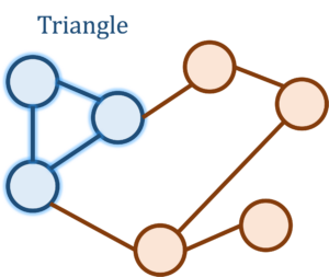
If there are $n$ people on the Facebook graph, then the natural algorithm of iterating over all ${n \choose 3} \approx n^3/6$ triplets and checking whether they form a triangle is far too computationally costly for the billions of Facebook accounts. Somehow, we want to do much faster than this, and to achieve this speed we would be willing to settle for an estimate of the triangle count up to some error.

There are many approaches to this problem, but let’s describe a particularly surprising algorithm. Let $A$ be an $n\times n$ matrix where the $ij$ th entry of $A$ is $1$ if users $i$ and $j$ are friends and $0$ otherwise¹; this matrix is called the adjacency matrix of the Facebook graph. A fact from graph theory is that the $ij$ th entry of the cube $A^3$ of the matrix $A$ counts the number of paths from user $i$ to user $j$ of length three.² In particular, the $ii$ th entry of $A^3$ denotes the number of paths from $i$ to itself of length $3$ , which is twice the number of triangles incident on $i$ . (The paths $i\to j \to k \to i$ and $i\to k \to j\to i$ are both counted as paths of length 3 for a triangle consisting of $i$ , $j$ , and $k$ .) Therefore, the trace of $A^3$ , equal to the sum of its diagonal entries, is six times the number of triangles: The $ii$ th entry of $A^3$ is twice the number of triangles incident on $i$ and each triangle $(i,j,k)$ is counted thrice in the $ii$ th, $jj$ th, and $kk$ th entries of $A^3$ . In summary, we have

$\begin{equation*} \mbox{\# triangles} = \frac{1}{6} \operatorname{tr} A^3. \end{equation*}$

Therefore, the triangle counting problem is equivalent to computing the trace of $A^3$ . Unfortunately, the problem of computing $A^3$ is, in general, very computationally costly. Therefore, we seek ways of estimating the trace of a matrix without forming it.

Randomized Trace Estimation

Motivated by the triangle counting problem from the previous section, we consider the problem of estimating the trace of a matrix $M$ . We assume that we only have access to the matrix $M$ through matrix–vector products; that is, we can efficiently compute $Mx$ for a vector $x$ . For instance, in the previous example, the Facebook graph has many fewer friend relations (edges) $m$ than the maximum possible amount of ${n\choose 2} \approx n^2/2$ . Therefore, the matrix $A$ is sparse; in particular, matrix–vector multiplications with $A$ can be computed in around $m$ operations. To compute matrix–vector products $Mx$ with $M = A^3$ , we simply compute matrix–vector products with $A$ three times, $x \mapsto Ax \mapsto A(Ax) \mapsto A(A(Ax)) = A^3x$ .

Here’s a very nifty idea to estimate the trace of $M$ using only matrix–vector products, originally due to Didier A. Girard and Michael F. Hutchinson. Choose $x$ to be a random vector whose entries are independent $\pm 1$ -values, where each value $+1$ and $-1$ occurs with equal $1/2$ probability. Then if one forms the expression $x^\top M x = \sum_{i,j=1}^n M_{ij} x_i x_j$ . Since the entries of $x_i$ and $x_j$ are independent, the expectation of $x_ix_j$ is $0$ for $i\ne j$ and $1$ for $i = j$ . Consequently, by linearity of expectation, the expected value of $x^\top M x$ is

$\begin{equation*} \mathbb{E} \, x^\top M x = \sum_{i,j=1}^n M_{ij} \mathbb{E} [x_ix_j] = \sum_{i = 1}^n M_{ii} = \operatorname{tr}(M). \end{equation*}$

The average value of $x^\top M x$ is equal to the trace of $M$ ! In the language of statistics, we might say that $x^\top M x$ is an unbiased estimator for $\operatorname{tr}(M)$ . Thus, the efficiently computable quantity $x^\top M x$ can serve as a (crude) estimate for $\operatorname{tr}(M)$ .

While the expectation of $x^\top Mx$ equals $\operatorname{tr}(M)$ , any random realization of $x^\top M x$ can deviate from $\operatorname{tr}(M)$ by a non-neligible amount. Thus, to reduce the variability of the estimator $x^\top M x$ , it is appropriate to take an average of multiple copies of this random estimate. Specifically, we draw $k$ random vectors with independent random $\pm 1$ entries $x_1,\ldots,x_k$ and compute the averaged trace estimator

(1) $\begin{equation*} T_k := \frac{1}{k} \sum_{j=1}^k x_j^\top M x_j^{\vphantom{\top}}. \end{equation*}$

The $k$ -sample trace estimator $T_k$ remains an unbiased estimator for $\operatorname{tr}(M)$ , $\mathbb{E}\, T_k = \operatorname{tr}(M)$ , but with reduced variability. Quantitatively, the variance of $T_k$ is $k$ times smaller than the single-sample estimator $x^\top M x$ :

(2) $\begin{equation*} \operatorname{Var}(T_k) = \frac{1}{k} \operatorname{Var}(x^\top M x). \end{equation*}$

The Girard–Hutchinson trace estimator gives a natural way of estimating the trace of the matrix $M$ , a task which might otherwise be hard without randomness.³ For the trace estimator to be a useful tool, an important question remains: How many samples $k$ are needed to compute $\operatorname{tr}(M)$ to a given accuracy? Concentration inequalities answer questions of this nature.

Concentration Inequalities

A concentration inequality provides a bound on the probability a random quantity is significantly larger or smaller than its typical value. Concentration inequalities are useful because they allow us to prove statements like “With at least 99% probability, the randomized trace estimator with 100 samples produces an approximation of the trace which is accurate up to error no larger than $0.001$ .” In other words, concentration inequalities can provide quantitative estimates of the likely size of the error when a randomized algorithm is executed.

In this section, we shall introduce a handful of useful concentration inequalities, which we will apply to the randomized trace estimator in the next section. We’ll then discuss how these and other concentration inequalities can be derived in the following section.

Markov’s Inequality

Markov’s inequality is the most fundamental concentration inequality. When used directly, it is a blunt instrument, requiring little insight to use and producing a crude but sometimes useful estimate. However, as we shall see later, all of the sophisticated concentration inequalities that will follow in this post can be derived from a careful use of Markov’s inequality.

The wide utility of Markov’s inequality is a consequence of the minimal assumptions needed for its use. Let $X$ be any nonnegative random variable. Markov’s inequality states that the probability that $X$ exceeds a level $t > 0$ is bounded by the expected value of $X$ over $t$ . In equations, we have

(3) $\begin{equation*} \mathbb{P} \left\{ X \ge t \right\} \le \frac{\mathbb{E} \, X}{t}. \end{equation*}$

We stress the fact that we make no assumptions on how the random quantity $X$ is generated other than that $X$ is nonnegative.

As a short example of Markov’s inequality, suppose we have a randomized algorithm which takes one second on average to run. Markov’s inequality then shows that the probability the algorithm takes more than 100 seconds to run is at most $1/100 = 1\%$ . This small example shows both the power and the limitation of Markov’s inequality. On the negative side, our analysis suggests that we might have to wait as much as 100 times the average runtime for the algorithm to complete running with 99% probability; this large huge multiple of 100 seems quite pessimistic. On the other hand, we needed no information whatsoever about how the algorithm works to do this analysis. In general, Markov’s inequality cannot be improved without more assumptions on the random variable $X$ .⁴

Chebyshev’s Inequality and Averages

The variance of a random variable describes the expected size of a random variable’s deviation from its expected value. As such, we would expect that the variance should provide a bound on the probability a random variable is far from its expectation. This intuition indeed is correct and is manifested by Chebyshev’s inequality. Let $X$ be a random variable (with finite expected value) and $t > 0$ . Chebyshev’s inequality states that the probability that $X$ deviates from its expected value by more than $t$ is at most $\operatorname{Var}(X)/t^2$ :

(4) $\begin{equation*} \mathbb{P} \left\{ \left| X - \mathbb{E} \, X \right| \ge t \right\} \le \frac{\operatorname{Var}(X)}{t^2}. \end{equation*}$

Chebyshev’s inequality is frequently applied to sums or averages of independent random quantities. Suppose $X_1,\ldots,X_n$ are independent and identically distributed random variables with mean $\mu$ and variance $\sigma^2$ and let $\overline{X}$ denote the average

$\begin{equation*} \overline{X} = \frac{X_1 + \cdots + X_n}{n}. \end{equation*}$

Since the random variables $X_1,\ldots,X_n$ are independent,⁵ the properties of variance entail that

$\begin{equation*} \operatorname{Var}(\overline{X}) = \operatorname{Var}\left( \frac{1}{n} X_1 + \cdots + \frac{1}{n} X_n \right) = \frac{1}{n^2} \operatorname{Var}(X_1) + \cdots + \frac{1}{n^2} \operatorname{Var}(X_n) = \frac{\sigma^2}{n}, \end{equation*}$

where we use the fact that $\operatorname{Var}(X_1) = \cdots = \operatorname{Var}(X_n) = \sigma^2$ . Therefore, by Chebyshev’s inequality,

(5) $\begin{equation*} \mathbb{P} \left\{ \left| \overline{X} - \mu \right| \ge t \right\} \le \frac{\sigma^2}{nt^2}. \end{equation*}$

Suppose we want to estimate the mean $\mu$ by $\overline{X}$ up to error $\epsilon$ and are willing to tolerate a failure probability of $\delta$ . Then setting the right-hand side of (5) to $\delta$ , Chebyshev’s inequality suggests that we need at most

(6) $\begin{equation*} n = \sigma^2\cdot \frac{1/\delta}{\epsilon^2} \end{equation*}$

samples to achieve this goal.

Exponential Concentration: Hoeffding and Bernstein

How happy should we be with the result (6) of applying Chebyshev’s inequality the average $\overline{X}$ ? The central limit theorem suggests that $\overline{X}$ should be approximately normally distributed with mean $\mu$ and variance $\sigma^2/n$ . Normal random variables have an exponentially small probability of being more than a few standard deviations above their mean, so it is natural to expect this should be true of $\overline{X}$ as well. Specifically, we expect a bound roughly like

(7) $\begin{equation*} \mathbb{P} \left\{ \left| \overline{X} - \mu \right| \ge t \right\} \stackrel{?}{\lessapprox} \exp\left(-\frac{nt^2}{2\sigma^2}\right). \end{equation*}$

Unfortunately, we don’t have a general result quite this nice without additional assumptions, but there are a diverse array of exponential concentration inequalities available which are quite useful in analyzing sums (or averages) of independent random variables that appear in applications.

Hoeffding’s inequality is one such bound. Let $X_1,\ldots,X_n$ be independent (but not necessarily identically distributed) random variables and consider the average $\overline{X} = (X_1 + \cdots + X_n)/n$ . Hoeffding’s inequality makes the assumption that the summands are bounded, say within an interval $[a,b]$ .⁶ Hoeffding’s inequality then states that

(8) $\begin{equation*} \mathbb{P}\left\{ \left|\overline{X} - \mathbb{E} \, \overline{X}\right| \ge t \right\} \le 2 \exp\left( -\frac{2nt^2}{(b-a)^2} \right). \end{equation*}$

Hoeffding’s inequality is quite similar to the ideal concentration result (7) except with the variance $\sigma^2 = n\operatorname{Var}(\overline{X})$ replaced by the potentially much larger quantity⁷ $(b-a)^2/4$ .

Bernstein’s inequality fixes this deficit in Hoeffding’s inequality at a small cost. Now, instead of assuming $X_1,\ldots,X_n$ are bounded within the interval $[a,b]$ , we make the alternate boundedness assumption $|X_i - \mathbb{E}\, X_i| \le B$ for every $1\le i\le n$ . We continue to denote $\sigma^2 = n\operatorname{Var}(\overline{X})$ so that if $X_1,\ldots,X_n$ are identically distributed, $\sigma^2$ denotes the variance of each of $X_1,\ldots,X_n$ . Bernstein’s inequality states that

(9) $\begin{equation*} \mathbb{P}\left\{ \left|\overline{X} - \mathbb{E} \, \overline{X}\right| \ge t \right\} \le 2 \exp\left( -\frac{nt^2/2}{\sigma^2 + Bt/3} \right). \end{equation*}$

For small values of $t$ , Bernstein’s inequality yields exactly the kind of concentration that we would hope for from our central limit theorem heuristic (7). However, for large values of $t$ , we have

$\begin{equation*} \mathbb{P}\left\{ \left|\overline{X} - \mathbb{E} \, \overline{X}\right| \ge t \right\} \stackrel{\mbox{large $t$}}{\lessapprox} 2 \exp\left( -\frac{3nt}{2B} \right), \end{equation*}$

which is exponentially small in $t$ rather than $t^2$ . We conclude that Bernstein’s inequality provides sharper bounds then Hoeffding’s inequality for smaller values of $t$ but weaker bounds for larger values of $t$ .

Chebyshev vs. Hoeffding vs. Bernstein

Let’s return to the situation where we seek to estimate the mean $\mu$ of independent and identically distributed random variables $X_1,\ldots,X_n$ each with variance $\sigma^2$ by using the averaged value $\overline{X} = (X_1 + \cdots + X_n)/n$ . Our goal is to bound how many samples $n$ we need to estimate $\mu$ up to error $\epsilon$ , $| \overline{X} - \mu | \le \epsilon$ , except with failure probability at most $\delta$ . Using Chebyshev’s inequality, we showed that (see (7))

$\begin{equation*} n \ge \sigma^2\cdot \frac{1/\delta}{\epsilon^2} \mbox{ suffices}. \end{equation*}$

Now, let’s try using Hoeffding’s inequality. Suppose that $X_1,\ldots,X_n$ are bounded in the interval $[a,b]$ . Then Hoeffding’s inequality (8) shows that

$\begin{equation*} n \ge \frac{(b-a)^2}{4}\cdot \frac{2\log(2/\delta)}{\epsilon^2} \mbox{ suffices}. \end{equation*}$

Bernstein’s inequality states that if $X_1,\ldots,X_n$ lie in the interval $[\mu-B,\mu+B]$ for every $1\le i \le n$ , then

(10) $\begin{equation*} n \ge \sigma^2 \cdot \frac{2\log(2/\delta)}{\epsilon^2} + B\cdot \frac{2/3\cdot\log(2/\delta)}{\epsilon} \mbox{ suffices}. \end{equation*}$

Hoeffding’s and Bernstein’s inequality show that we need $n$ roughly proportional to $\tfrac{\log(1/\delta)}{\epsilon^2}$ samples are needed rather than proportional to $\tfrac{1/\delta}{\epsilon^2}$ . The fact that we need proportional to $1/\epsilon^2$ samples to achieve error $\epsilon$ is a consequence of the central limit theorem and is something we would not be able to improve with any concentration inequality. What exponential concentration inequalities allow us to do is to improve the dependence on the failure probability from proportional to $1/\delta$ to $\log(1/\delta)$ , which is a huge improvement.

Hoeffding’s and Bernstein’s inequalities both have a small drawback. For Hoeffding’s inequality, the constant of proportionality is $(b-a)^2/4$ rather than the true variance $\sigma^2$ of the summands. Bernstein’s inequality gives us the “correct” constant of proportionality $\sigma^2$ but adds a second term proportional to $\tfrac{\log(1/\delta)}{\epsilon}$ ; for small values of $\epsilon$ , this term is dominated by the term proportional to $\tfrac{\log(1/\delta)}{\epsilon^2}$ but the second term can be relevant for larger values of $\epsilon$ .

There are a panoply of additional concentration inequalities than the few we’ve mentioned. We give a selected overview in the following optional section.

Other Concentration Inequalities

There are a handful more exponential concentration inequalities for sums of independent random variables such as Chernoff’s inequality (very useful for somes of bounded, positive random variables) and Bennett’s inequality. There are also generalizations of Hoeffding’s, Chernoff’s, and Bernstein’s inequalities for unbounded random variables with subgaussian and subexponential tail decay; these results are documented in Chapter 2 of Roman Vershynin’s excellent book High-Dimensional Probability.

One can also generalize concentration inequalities to so-called martingale sequences, which can be very useful for analyzing adaptive algorithms. These inequalities can often have the advantage of bounding the probability that a martingale sequence ever deviates by some amount from its applications; these results are called maximal inequalities. Maximal analogs of Markov’s and Chebyshev’s inequalities are given by Ville’s inequality and Doob’s inequality. Exponential concentration inequalities include the Hoeffding–Azuma inequality and Freedman’s inequality.

Finally, we note that there are many concentration inequalities for functions of independent random variables other than sums, usually under the assumption that the function is Lipschitz continuous. There are exponential concentration inequalities for functions with “bounded differences”, functions of Gaussian random variables, and convex functions of bounded random variables. References for these results include Chapters 3 and 4 of the lecture notes Probability in High Dimension by Ramon van Handel and the comprehensive monograph Concentration Inequalities by Stéphane Boucheron, Gábor Lugosi, and Pascal Massart.

Analysis of Randomized Trace Estimation

Let us apply some of the concentration inequalities we introduced in last section to analyze the randomized trace estimator. Our goal is not to provide the best possible analysis of the trace estimator,⁸ but to demonstrate how the general concentration inequalities we’ve developed can be useful “out of the box” in analyzing algorithms.

In order to apply Chebyshev’s and Berstein’s inequalities, we shall need to compute or bound the variance of the single-sample trace estimtor $x^\top Mx$ , where $x$ is a random vector of independent $\pm 1$ -values. This is a straightforward task using properties of the variance:

$\begin{equation*} \operatorname{Var}(x^\top M x) = \operatorname{Var}\left( 2\sum_{i< j} M_{ij} x_i x_j \right) = 4\sum_{i\ne j, \: k\ne \ell} M_{ij} M_{k\ell} \operatorname{Cov}(x_ix_j,x_kx_\ell) = 4\sum_{i < j} M_{ij}^2 \le 2 \|M\|_{\rm F}^2 \end{equation*}$

Here, $\operatorname{Cov}$ is the covariance and $\|\cdot\|_{\rm F}$ is the matrix Frobenius norm. Chebyshev’s inequality (5), then gives

$\begin{equation*} \mathbb{P} \left\{ \left|T_k - \operatorname{tr}(M)\right| \ge t \right\} \le \frac{2\|M\|_{\rm F}^2}{kt^2}. \end{equation*}$

Let’s now try applying an exponential concentration inequality. We shall use Bernstein’s inequality, for which we need to bound $|x^\top M x - \operatorname{tr}(M)|$ . By the Courant–Fischer minimax principle, we know that $x^\top M x$ is between $\lambda_{\rm min}(M) \cdot \|x\|^2$ and $\lambda_{\rm max} (M)\cdot\|x\|^2$ where $\lambda_{\rm min}(M)$ and $\lambda_{\rm max}(M)$ are the smallest and largest eigenvalues of $M$ and $\|x\|$ is the Euclidean norm of the vector $x$ . Since all the entries of $x$ have absolute value $1$ , we have $\|x\| = \sqrt{n}$ so $x^\top M x$ is between $n\lambda_{\rm min}(M)$ and $n\lambda_{\rm max}(M)$ . Since the trace equals the sum of the eigenvalues of $M$ , $\operatorname{tr}(M)$ is also between $n\lambda_{\rm min}(M)$ and $n\lambda_{\rm max}(M)$ . Therefore,

$\begin{equation*} \left| x^\top M x - \operatorname{tr}(M) \right| \le n \left( \lambda_{\rm max}(M) - \lambda_{\rm min}(M)\right) \le 2 n \|M\|, \end{equation*}$

where $\|\cdot\|$ denotes the matrix spectral norm. Therefore, by Bernstein’s inequality (9), we have

$\begin{equation*} \mathbb{P} \left\{ \left| T_k - \operatorname{tr}(M) \right| \ge t \right\} \le 2\exp\left( -\frac{kt^2}{4\|M\|_{\rm F}^2 + 4/3\cdot tn\|M\|} \right). \end{equation*}$

In particular, (10) shows that

$\begin{equation*} k \ge \left( \frac{4\|M\|_{\rm F}^2}{\epsilon^2} + \frac{4n\|M\|}{3\epsilon} \right) \log \left(\frac{2}{\delta} \right) \end{equation*}$

samples suffice to estimate $\operatorname{tr}(M)$ to error $\epsilon$ with failure probability at most $\delta$ . Concentration inequalities easily furnish estimates for the number of samples needed for the randomized trace estimator.

We have now accomplished our main goal of using concentration inequalities to analyze the randomized trace estimator, which in turn can be used to solve the triangle counting problem. We leave some additional comments on trace estimation and triangle counting in the following bonus section.

More on Trace Estimation and Triangle Counting

To really complete the analysis of the trace estimator in an application (e.g., triangle counting), we would need to obtain bounds on $\|M\|_{\rm F}$ and $\|M\|$ . Since we often don’t know good bounds for $\|M\|_{\rm F}$ and $\|M \|$ , one should really use the trace estimator together with an a posteriori error estimates for the trace estimator, which provide a confidence interval for the trace rather than a point estimate; see sections 4.5 and 4.6 in this survey for details.

One can improve on the Girard–Hutchinson trace estimator by using a variance reduction technique. One such variance reduction technique was recently proposed under the name Hutch++, extending ideas by Arjun Singh Gambhir, Andreas Stathopoulos, and Kostas Orginos and Lin Lin. In effect, these techniques improve the number of samples $k$ needed to estimate the trace of a positive semidefinite matrix $A$ to relative error $\epsilon$ to proportional to $1/\epsilon$ down from $1/\epsilon^2$ .

Several algorithms have been proposed for triangle counting, many of them randomized. This survey gives a comparison of different methods for the triangle counting problem, and also describes more motivation and applications for the problem.

Deriving Concentration Inequalities

Having introduced concentration inequalities and applied them to the randomized trace estimator, we now turn to the question of how to derive concentration inequalities. Learning how to derive concentration inequalities is more than a matter of mathematical completeness since one can often obtain better results by “hand-crafting” a concentration inequality for a particular application rather than applying a known concentration inequality. (Though standard concentration inequalities like Hoeffding’s and Bernstein’s often give perfectly adequate answers with much less work.)

Markov’s Inequality

At the most fundamental level, concentration inequalities require us to bound a probability by an expectation. In achieving this goal, we shall make a simple observation: The probability that $X$ is larger than or equal to $t$ is the expectation of a random variable $\mathbf{1}_{[t,\infty)}(X)$ .⁹ Here, $\mathbf{1}_{[t,\infty)}(\cdot)$ is an indicator function which outputs one if its input is larger than or equal to $t$ and zero otherwise.

As promised, the probability $X$ is larger than $t$ is the expectation of $\mathbf{1}_{[t,\infty)}(X)$ :

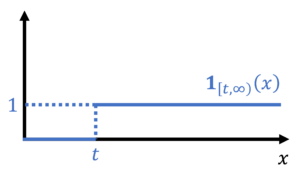
(11) $\begin{equation*} \mathbb{P}\{X \ge t \} = \mathbb{E}[\mathbf{1}_{[t,\infty)}(X)]. \end{equation*}$

We can now obtain bounds on the probability that $X\ge t$ by bounding its corresponding indicator function. In particular, we have the inequality

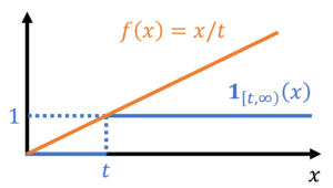
(12) $\begin{equation*} \mathbf{1}_{[t,\infty)}(x) \le \frac{x}{t} \mbox{ for every } x\ge 0. \end{equation*}$

Since $X$ is nonnegative, combining equations (11) and (12) gives Markov’s inequality:

$\begin{equation*} \mathbb{P}\{ X \ge t \} = \mathbb{E}[\mathbf{1}_{[t,\infty)}(X)] \le \mathbb{E} \left[ \frac{X}{t} \right] = \frac{\mathbb{E} X}{t}. \end{equation*}$

Chebyshev’s Inequality

Before we get to Chebyshev’s inequality proper, let’s think about how we can push Markov’s inequality further. Suppose we find a bound on the indicator function $\mathbf{1}_{[t,\infty)}(\cdot)$ of the form

(13) $\begin{equation*} \mathbf{1}_{[t,\infty)}(x) \le f(x) \mbox{ for all } x\ge 0. \end{equation*}$

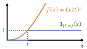
A bound of this form immediately to bounds on $\mathbb{P} \{X \ge t\}$ by (11). To obtain sharp and useful bounds on $\mathbb{P}\{X\ge t\}$ we seek bounding functions $f(\cdot)$ in (13) with three properties:

For $x\in[0, t)$ , $f(x)$ should be close to zero,
For $x\in [t,\infty)$ , $f(x)$ should be close to one, and
We need $\mathbb{E} \, f(X)$ to be easily computable or boundable.

These three objectives are in tension with each other. To meet criterion 3, we must restrict our attention to pedestrian functions $f(\cdot)$ such as powers $f(x) = (x/t)^\theta$ or exponentials $f(x) = \exp(\theta (x-t))$ for which we have hopes of computing or bounding $\mathbb{E} \, f(X)$ for random variables $X$ we encounter in practical applications. But these candidate functions $f(\cdot)$ have the undesirable property that making the function smaller on $[0, t)$ (by increasing $\theta$ ) to meet point 1 makes the function larger on $(t,\infty)$ , detracting from our ability to achieve point 2. We shall eventually come up with a best-possible resolution to this dilemma by formulating this as an optimization problem to determine the best choice of the parameter $\theta > 0$ to obtain the best possible candidate function of the given form.

Before we get ahead of ourselves, let us use a specific choice for $f(\cdot)$ different than we used to prove Markov’s inequality. We readily verify that $f(x) = (x/t)^2$ satisfies the bound (13), and thus by (12),

(14) $\begin{equation*} \mathbb{P} \{ X \ge t \} \le \mathbb{E} \left( \frac{X}{t} \right)^2 = \frac{\mathbb{E} X^2}{t^2}. \end{equation*}$

This inequality holds for any nonnegative random variable $X$ . In particular, now consider a random variable $X$ which we do not assume to be nonnegative. Then $X$ ‘s deviation from its expectation, $|X-\mathbb{E} X|$ , is a nonnegative random variable. Thus applying (14) gives

$\begin{equation*}\mathbb{P} \{ |X - \mathbb{E} X| \ge t \} \le \frac{\mathbb{E} | X - \mathbb{E} X|^2}{t^2} = \frac{\operatorname{Var}(X)}{t^2}. \end{equation*}$

We have derived Chebyshev’s inequality! Alternatively, one can derive Chebyshev’s inequality by noting that $|X-\mathbb{E} X| \ge t$ if, and only if, $|X-\mathbb{E} X|^2 \ge t^2$ . Therefore, by Markov’s inequality,

$\begin{equation*} \mathbb{P} \{ |X - \mathbb{E} X| \ge t \} = \mathbb{P} \{ |X - \mathbb{E} X|^2 \ge t^2 \} \le \frac{\mathbb{E} | X - \mathbb{E} X|^2}{t^2} = \frac{\operatorname{Var}(X)}{t^2}. \end{equation*}$

The Laplace Transform Method

We shall now realize the plan outlined earlier where we shall choose an optimal bounding function $f(\cdot)$ from the family of exponential functions $f(x) = \exp(\theta(x-t))$ , where $\theta > 0$ is a parameter which we shall optimize over. This method shall allow us to derive exponential concentration inequalities like Hoeffding’s and Bernstein’s. Note that the exponential function $f(x) = \exp(\theta(x-t))$ bounds the indicator function $\mathbf{1}_{[t,\infty)}(\cdot)$ for all real numbers $x$ , so we shall no longer require the random variable $X$ to be nonnegative. Therefore, by (11),

(15) $\begin{equation*} \mathbb{P} \{ X \ge t \} \le \mathbb{E} \exp\left(\theta (X-t)\right) = \exp(-\theta t) \,\mathbb{E} \exp(\theta X) = \exp\left(-\theta t + \log \mathbb{E} \exp(\theta X) \right). \end{equation*}$

The functions

$\begin{equation*} m_X(\theta) = \mathbb{E} \exp(\theta X), \quad \xi_X(\theta) = \log \mathbb{E} \exp(\theta X) = \log m_X(\theta) \end{equation*}$

are known as the moment generating function and cumulant generating function of the random variable $X$ .¹⁰ With these notations, (15) can be written

(16) $\begin{equation*} \mathbb{P} \{ X \ge t \} \le\exp(-\theta t) m_X(\theta) = \exp\left(-\theta t + \xi_X(\theta) \right). \end{equation*}$

The moment generating function coincides with the Laplace transform $\mathbb{E} \exp(-\theta X) = m_X(-\theta)$ up to the sign of the parameter $\theta$ , so one name for this approach to deriving concentration inequalities is the Laplace transform method. (This method is also known as the Cramér–Chernoff method.)

The cumulant generating function has an important property for deriving concentration inequalities for sums or averages of independent random variables: If $X_1,\ldots,X_n$ are independent random variables, than the cumulant generating function is additive:¹¹

(17) $\begin{equation*} \xi_{X_1 + \cdots + X_n}(\theta) = \xi_{X_1}(\theta) + \cdots + \xi_{X_n}(\theta). \end{equation*}$

Proving Hoeffding’s Inequality

For us to use the Laplace transform method, we need to either compute or bound the cumulant generating function. Since we are interested in general concentration inequalities which hold under minimal assumptions such as boundedness, we opt for the latter. Suppose $a\le X \le b$ and consider the cumulant generating function of $Y:=X-\mathbb{E}X$ . Then one can show the cumulant generating function bound¹²

(18) $\begin{equation*} \xi_Y(\theta) \le \frac{1}{8} \theta^2(b-a)^2. \end{equation*}$

Using the additivity of the cumulant generating function (17), we obtain the bound

$\begin{equation*} \xi_{\overline{X} - \mathbb{E} \overline{X}}(\theta) = \xi_{X_1/n- \mathbb{E}X_1/n}(\theta) + \cdots + \xi_{X_n/n- \mathbb{E}X_n/n}(\theta) \le \frac{1}{n} \cdot \frac{1}{8} \theta^2(b-a)^2. \end{equation*}$

Plugging this into the probability bound (16), we obtain the concentration bound

(19) $\begin{equation*} \mathbb{P} \left\{ \overline{X} - \mathbb{E} \overline{X} \ge t \right\} \le \exp \left( - \theta t +\frac{1}{n} \cdot \frac{1}{8} \theta^2(b-a)^2 \right). \end{equation*}$

We want to obtain the smallest possible upper bound on this probability, so it behooves us to pick the value of $\theta > 0$ which makes the right-hand side of this inequality as small as possible. To do this, we differentiate the contents of the exponential and set to zero, obtaining

$\begin{equation*} \frac{\mathrm{d}}{\mathrm{d} \theta} \left( - \theta t + \frac{1}{n} \cdot \frac{1}{8} \theta^2(b-a)^2\right) = - t + \frac{1}{n} \cdot \frac{1}{4} (b-a)^2 \theta = 0\implies \theta = \frac{4nt}{(b-a)^2} \end{equation*}$

Plugging this value for $\theta$ into the bound (19) gives A bound for $\overline{X}$ being larger than $\mathbb{E}\overline{X} + t$ :

(20) $\begin{equation*} \mathbb{P} \left\{ \overline{X} - \mathbb{E} \overline{X} \ge t \right\} \le \exp \left( - \frac{2nt^2}{(b-a)^2} \right). \end{equation*}$

To get the bound on $\overline{X}$ being smaller than $\mathbb{E}\overline{X} - t$ , we can apply a small trick. If we apply (20) to the summands $-X_1,-X_2,\ldots,-X_n$ instead of $X_1,\ldots,X_n$ , we obtain the bounds

(21) $\begin{equation*} \mathbb{P} \left\{ \overline{X} - \mathbb{E} \overline{X} \le -t \right\} \le \exp \left( - \frac{2nt^2}{(b-a)^2} \right). \end{equation*}$

We can now combine the upper tail bound (19) with the lower tail bound (21) to obtain a “symmetric” bound on the probability that $|\overline{X} - \mathbb{E}\overline{X}| \ge t$ . The means of doing often this goes by the fancy name union bound, but the idea is very simple:

$\begin{equation*} \mathbb{P}(\textnormal{A happens or B happens} )\le \mathbb{P}(\textnormal{A happens}) + \mathbb{P}(\textnormal{B happens}). \end{equation*}$

Thus, applying this union bound idea with the upper and lower tail bounds (20) and (21), we obtain Hoeffding’s inequality, exactly as it appeared above as (8):

$\begin{align*} \mathbb{P}\left\{ |\overline{X} - \mathbb{E}\overline{X}| \ge t \right\} &= \mathbb{P}\left\{ \overline{X} - \mathbb{E}\overline{X} \ge t \textnormal{ or } \overline{X} - \mathbb{E}\overline{X} \le -t \right\}\\ &\le \mathbb{P} \left\{ \overline{X} - \mathbb{E} \overline{X} \ge t \right\} + \mathbb{P} \left\{ \overline{X} - \mathbb{E} \overline{X} \le -t \right\}\\ &\le 2\exp \left( - \frac{2nt^2}{(b-a)^2} \right). \end{align*}$

Voilà! Hoeffding’s inequality has been proven! Bernstein’s inequality is proven essentially the same way except that, instead of (17), we have the cumulant generating function bound

$\begin{equation*} \xi_Y(\theta) = \frac{(\theta^2/2)\Var(Y)}{1-|\theta|/3} \end{equation*}$

for a random variable $Y$ with mean zero and satisfying the bound $|Y| \le B$ .

Upshot: Randomness can be a very effective tool for solving computational problems, even those which seemingly no connection to probability like triangle counting. Concentration inequalities are a powerful tool for assessing how many samples are needed for an algorithm based on random sampling to work. Some of the most useful concentration inequalities are exponential concentration inequalities like Hoeffding and Bernstein, which show that an average of bounded random quantities are close to their average except with exponentially small probability.

Distribution	Variance (divided by $\tr(A)^2$ )
Gaussian	$2.0\times 10^{-3}$
Sphere	$6.7\times 10^{-6}$
Random signs	$6.7\times 10^{-6}$