Low-Rank Approximation Toolbox: Nyström, Cholesky, and Schur

In the last post, we looked at the Nyström approximation to an $N\times N$ positive semidefinite (psd) matrix $A$ . A special case was the column Nyström approximation, defined to be¹

(Nys) $\hat{A} = A(:,S) \, A(S,S)^{-1} \, A(S,:),$

where $S = \{s_1,\ldots,s_k\} \subseteq \{1,2,\ldots,N\}$ identifies a subset of $k$ columns of $A$ . Provided $k\ll N$ , this allowed us to approximate all $N^2$ entries of the matrix $A$ using only the $kN$ entries in columns $s_1,\ldots,s_k$ of $A$ , a huge savings of computational effort!

With the column Nyström approximation presented just as such, many questions remain:

Why this formula?
Where did it come from?
How do we pick the columns $s_1,\ldots,s_k$ ?
What is the residual $A - \hat{A}$ of the approximation?

In this post, we will answer all of these questions by drawing a connection between low-rank approximation by Nyström approximation and solving linear systems of equations by Gaussian elimination. The connection between these two seemingly unrelated areas of matrix computations will pay dividends, leading to effective algorithms to compute Nyström approximations by the (partial) Cholesky factorization of a positive (semi)definite matrix and an elegant description of the residual of the Nyström approximation as the Schur complement.

Cholesky: Solving Linear Systems

Suppose we want solve the system of linear equations $Ax = b$ , where $A$ is a real $N\times N$ invertible matrix and $b$ is a vector of length $N$ . The standard way of doing this in modern practice (at least for non-huge matrices $A$ ) is by means of Gaussian elimination/LU factorization. We factor the matrix $A$ as a product $A = LU$ of a lower triangular matrix $L$ and an upper triangular matrix $U$ .² The system $Ax = b$ is solved by first solving $Ly = b$ for $y$ and then $Ux = y$ for $x$ ; the triangularity of $L$ and $U$ make solving the associated systems of linear equations easy.

For real symmetric positive definite matrix $A$ , a simplification is possible. In this case, one can compute an LU factorization where the matrices $L$ and $U$ are transposes of each other, $U = L^\top$ . This factorization $A = LL^\top$ is known as a Cholesky factorization of the matrix $A$ .

The Cholesky factorization can be easily generalized to allow the matrix $A$ to be complex-valued. For a complex-valued positive definite matrix $A$ , its Cholesky decomposition takes the form $A = LL^*$ , where $L$ is again a lower triangular matrix. All that has changed is that the transpose ${}^\top$ has been replaced by the conjugate transpose ${}^*$ . We shall work with the more general complex case going forward, though the reader is free to imagine all matrices as real and interpret the operation ${}^*$ as ordinary transposition if they so choose.

Schur: Computing the Cholesky Factorization

Here’s one way of computing the Cholesky factorization using recursion. Write the matrix $A$ in block form as

$A = \twobytwo{A_{11}}{A_{12}}{A_{21}}{A_{22}}.$

Our first step will be “block Cholesky factorize” the matrix $A$ , factoring $A$ as a product of matrices which are only block triangular. Then, we’ll “upgrade” this block factorization into a full Cholesky factorization.

The core idea of Gaussian elimination is to combine rows of a matrix to introduce zero entries. For our case, observe that multiplying the first block row of $A$ by $A_{21}A_{11}^{-1}$ and subtracting this from the second block row introduces a matrix of zeros into the bottom left block of $A$ . (The matrix $A_{11}$ is a principal submatrix of $A$ and is therefore guaranteed to be positive definite and thus invertible.³) In matrix language,

$\twobytwo{I}{0}{-A_{21}A_{11}^{-1}}{I}\twobytwo{A_{11}}{A_{12}}{A_{21}}{A_{22}} = \twobytwo{A_{11}}{A_{12}}{0}{A_{22} - A_{21}A_{11}^{-1}A_{12}}.$

Isolating $A$ on the left-hand side of this equation by multiplying by

$\twobytwo{I}{0}{-A_{21}A_{11}^{-1}}{I}^{-1} = \twobytwo{I}{0}{A_{21}A_{11}^{-1}}{I}$

yields the block triangular factorization

$A = \twobytwo{A_{11}}{A_{12}}{A_{21}}{A_{22}} = \twobytwo{I}{0}{A_{21}A_{11}^{-1}}{I} \twobytwo{A_{11}}{A_{12}}{0}{A_{22} - A_{21}A_{11}^{-1}A_{12}}.$

We’ve factored $A$ into block triangular pieces, but these pieces are not (conjugate) transposes of each other. Thus, to make this equation more symmetrical, we can further decompose

(1) $A = \twobytwo{A_{11}}{A_{12}}{A_{21}}{A_{22}} = \twobytwo{I}{0}{A_{21}A_{11}^{-1}}{I} \twobytwo{A_{11}}{0}{0}{A_{22} - A_{21}A_{11}^{-1}A_{12}} \twobytwo{I}{0}{A_{21}A_{11}^{-1}}{I}^*.$

This is a block version of the Cholesky decomposition of the matrix $A$ taking the form $A = LDL^*$ , where $L$ is a block lower triangular matrix and $D$ is a block diagonal matrix.

We’ve met the second of our main characters, the Schur complement

(Sch) $S = A_{22} - A_{21}A_{11}^{-1}A_{12}.$

This seemingly innocuous combination of matrices has a tendency to show up in surprising places when one works with matrices.⁴ It’s appearance in any one place is unremarkable, but the shear ubiquity of $A_{22} - A_{21}A_{11}^{-1}A_{12}$ in matrix theory makes it deserving of its special name, the Schur complement. To us for now, the Schur complement is just the matrix appearing in the bottom right corner of our block Cholesky factorization.

The Schur complement enjoys the following property:⁵

Positivity of the Schur complement: If $A=\twobytwo{A_{11}}{A_{12}}{A_{21}}{A_{22}}$ is positive (semi)definite, then the Schur complement $S = A_{22} - A_{21}A_{11}^{-1}A_{12}$ is positive (semi)definite.

As a consequence of this property, we conclude that both $A_{11}$ and $S$ are positive definite.

With the positive definiteness of the Schur complement in hand, we now return to our Cholesky factorization algorithm. Continue by recursively⁶ computing Cholesky factorizations of the diagonal blocks

$A_{11} = L_{11}^{\vphantom{*}}L_{11}^*, \quad S = L_{22}^{\vphantom{*}}L_{22}^*.$

Inserting these into the block $LDL^*$ factorization (1) and simplifying gives a Cholesky factorization, as desired:

$A = \twobytwo{L_{11}}{0}{A_{21}^{\vphantom{*}}(L_{11}^{*})^{-1}}{L_{22}}\twobytwo{L_{11}}{0}{A_{21}^{\vphantom{*}}(L_{11}^{*})^{-1}}{L_{22}}^* =: LL^*.$

Voilà, we have obtained a Cholesky factorization of a positive definite matrix $A$ !

By unwinding the recursions (and always choosing the top left block $A_{11}$ to be of size $1\times 1$ ), our recursive Cholesky algorithm becomes the following iterative algorithm: Initialize $L$ to be the zero matrix. For $j = 1,2,3,\ldots,N$ , perform the following steps:

Update $L$ . Set the $j$ th column of $L$ :
$L(j:N,j) \leftarrow A(j:N,j)/\sqrt{a_{jj}}.$
Update $A$ . Update the bottom right portion of $A$ to be the Schur complement:
$A(j+1:N,j+1:N)\leftarrow A(j+1:N,j+1:N) - \frac{A(j+1:N,j)A(j,j+1:N)}{a_{jj}}.$

This iterative algorithm is how Cholesky factorization is typically presented in textbooks.

Nyström: Using Cholesky Factorization for Low-Rank Approximation

Our motivating interest in studying the Cholesky factorization was the solution of linear systems of equations $Ax = b$ for a positive definite matrix $A$ . We can also use the Cholesky factorization for a very different task, low-rank approximation.

Let’s first look at things through the lense of the recursive form of the Cholesky factorization. The first step of the factorization was to form the block Cholesky factorization

$A = \twobytwo{I}{0}{A_{21}A_{11}^{-1}}{I} \twobytwo{A_{11}}{0}{0}{A_{22} - A_{21}A_{11}^{-1}A_{12}} \twobytwo{I}{0}{A_{21}A_{11}^{-1}}{I}^*.$

Suppose that we choose the top left $A_{11}$ block to be of size $k\times k$ , where $k$ is much smaller than $N$ . The most expensive part of the Cholesky factorization will be the recursive factorization of the Schur complement $A_{22} - A_{21}A_{11}^{-1} A_{12}$ , which is a large matrix of size $(N-k)\times (N-k)$ .

To reduce computational cost, we ask the provocative question: What if we simply didn’t factorize the Schur complement? Observe that we can write the block Cholesky factorization as a sum of two terms

(2) $A = \twobyone{I}{A_{21}{A_{11}^{-1}}} A_{11} \twobyone{I}{A_{22}{A_{11}^{-1}}}^* + \twobytwo{0}{0}{0}{A_{22}-A_{21}A_{11}^{-1}A_{12}}.$

We can use the first term of this sum as a rank- $k$ approximation to the matrix $A$ . The low-rank approximation, which we can write out more conveniently as

$\hat{A} = \twobyone{A_{11}}{A_{21}} A_{11}^{-1} \onebytwo{A_{11}}{A_{12}} = \twobytwo{A_{11}}{A_{12}}{A_{21}}{A_{21}A_{11}^{-1}A_{12}},$

is the column Nyström approximation (Nys) to $A$ associated with the index set $S = \{1,2,3,\ldots,k\}$ and is the final of our three titular characters. The residual of the Nyström approximation is the second term in (2), which is none other than the Schur complement (Sch), padded by rows and columns of zeros:

$A - \hat{A} = \twobytwo{0}{0}{0}{A_{22}-A_{21}A_{11}^{-1}A_{12}}.$

Observe that the approximation $\hat{A}$ is obtained from the process of terminating a Cholesky factorization midway through algorithm execution, so we say that the Nyström approximation results from a partial Cholesky factorization of the matrix $A$ .

Summing things up:

If we perform a partial Cholesky factorization on a positive (semi)definite matrix, we obtain a low-rank approximation known as the column Nyström approximation. The residual of this approximation is the Schur complement, padded by rows and columns of zeros.

The idea of obtaining a low-rank approximation from a partial matrix factorization is very common in matrix computations. Indeed, the optimal low-rank approximation to a real symmetric matrix is obtained by truncating its eigenvalue decomposition and the optimal low-rank approximation to a general matrix is obtained by truncating its singular value decomposition. While the column Nyström approximation is not the optimal rank- $k$ approximation to $A$ (though it does satisfy a weaker notion of optimality, as discussed in this previous post), it has a killer feature not possessed by the optimal approximation:

The column Nyström approximation is formed from only $k$ columns from the matrix $A$ . A column Nyström approximation approximates an $N\times N$ matrix by only reading a fraction of its entries!

Unfortunately there’s not a free lunch here. The column Nyström is only a good low-rank approximation if the Schur complement has small entries. In general, this need not be the case. Fortunately, we can improve our situation by means of pivoting.

Our iterative Cholesky algorithm first performs elimination using the entry in position $(1,1)$ followed by position $(2,2)$ and so on. There’s no need to insist on this exact ordering of elimination steps. Indeed, at each step of the Cholesky algorithm, we can choose whichever diagonal position $(j,j)$ that we want to perform elimination. The entry we choose to perform elimination with is called a pivot.

Obtaining good column Nyström approximations requires identifying the a good choice for the pivots to reduce the size of the entries of the Schur complement at each step of the algorithm. With general pivot selection, an iterative algorithm for computing a column Nyström approximation by partial Cholesky factorization proceeds as follows: Initialize an $N\times k$ matrix $F$ to store the column Nyström approximation $\hat{A} = FF^*$ , in factored form. For $j = 1,2,\ldots,k$ , perform the following steps:

Select pivot. Choose a pivot $s_j$ .
Update the approximation. $F(:,j) \leftarrow A(:,s_j) / \sqrt{a_{s_js_j}}$ .
Update the residual. $A \leftarrow A - \frac{A(:,s_j)A(s_j,:)}{a_{s_js_j}}$ .

This procedure results in the Nyström approximation (Nys) with column set $S = \{s_1,\ldots,s_k\}$ :

$\hat{A} = FF^* = A(:,S) \, A(S,S)^{-1} \, A(S,:).$

The pivoted Cholesky steps 1–3 requires updating the entire matrix $A$ at every step. With a little more cleverness, we can optimize this procedure to only update the entries of the matrix $A$ we need to form the approximation $\hat{A} = FF^*$ . See Algorithm 2 in this preprint of my coauthors and I for details.

How should we choose the pivots? Two simple strategies immediately suggest themselves:

Uniformly random. At each step $j$ , select $s_j$ uniformly at random from among the un-selected pivot indices.
Greedy.⁷ At each step $j$ , select $s_j$ according to the largest diagonal entry of the current residual $A$ :
$s_j = \argmax_{1\le k\le N} a_{kk}.$

The greedy strategy often (but not always) works well, and the uniformly random approach can work surprisingly well if the matrix $A$ is “incoherent”, with all rows and columns of the matrix possessing “similar importance”.

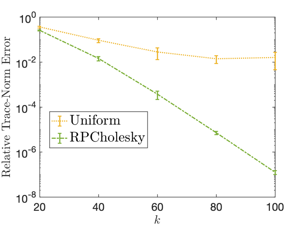
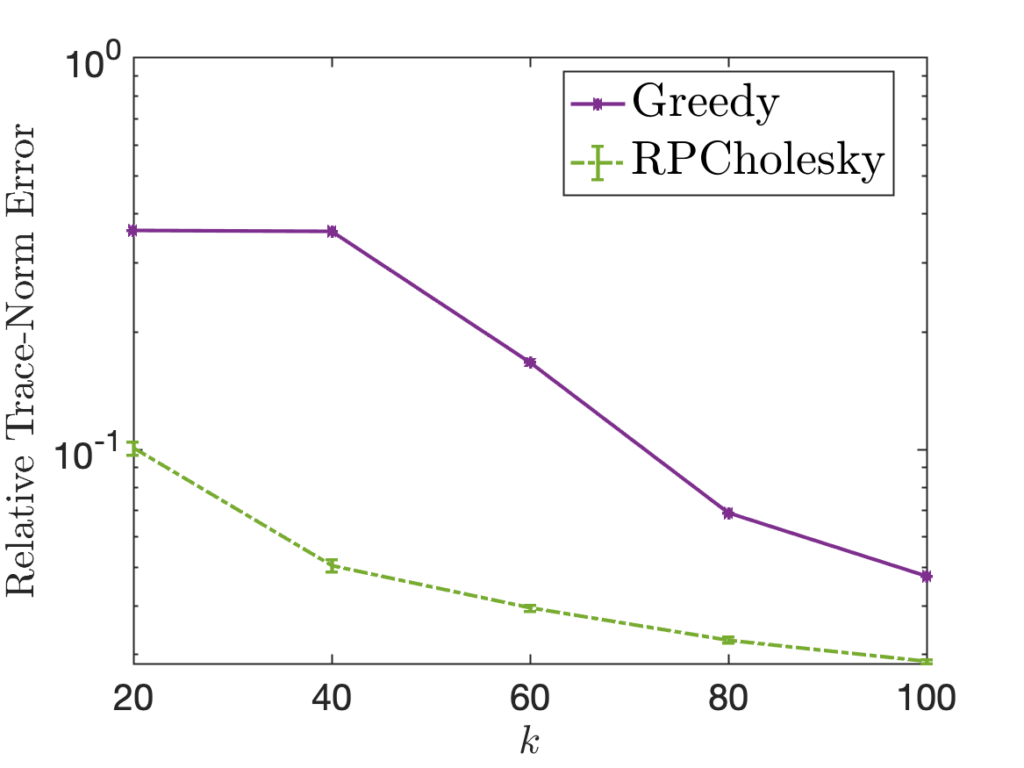
Despite often working fairly well, both the uniform and greedy schemes can fail significantly, producing very low-quality approximations. My research (joint with Yifan Chen, Joel A. Tropp, and Robert J. Webber) has investigated a third strategy striking a balance between these two approaches:

Diagonally weighted random. At each step $j$ , select $s_j$ at random according to the probability weights based on the current diagonal of the matrix
$\mathbb{P} \{ s_j = k \} = \frac{a_{kk}}{\operatorname{tr} A}.$

Our paper provides theoretical analysis and empirical evidence showing that this diagonally-weighted random pivot selection (which we call randomly pivoted Cholesky aka RPCholesky) performs well at approximating all positive semidefinite matrices $A$ , even those for which uniform random and greedy pivot selection fail. The success of this approach can be seen in the following examples (from Figure 1 in the paper), which shows RPCholesky can produce much smaller errors than the greedy and uniform methods.

Conclusions

In this post, we’ve seen that a column Nyström approximation can be obtained from a partial Cholesky decomposition. The residual of the approximation is the Schur complement. I hope you agree that this is a very nice connection between these three ideas. But beyond its mathematical beauty, why do we care about this connection? Here are my reasons for caring:

Analysis. Cholesky factorization and the Schur complement are very well-studied in matrix theory. We can use known facts about Cholesky factorization and Schur complements to prove things about the Nyström approximation, as we did when we invoked the positivity of the Schur complement.
Algorithms. Cholesky factorization-based algorithms like randomly pivoted Cholesky are effective in practice at producing high-quality column Nyström approximations.

On a broader level, our tale of Nyström, Cholesky, and Schur demonstrates that there are rich connections between low-rank approximation and (partial versions of) classical matrix factorizations like LU (with partial pivoting), Cholesky, QR, eigendecomposition, and SVD for to full-rank matrices. These connections can be vital to analyzing low-rank approximation algorithms and developing improvements.

Low-Rank Approximation Toolbox: Nyström, Cholesky, and Schur

Cholesky: Solving Linear Systems

Schur: Computing the Cholesky Factorization

Nyström: Using Cholesky Factorization for Low-Rank Approximation

Conclusions

2 thoughts on “Low-Rank Approximation Toolbox: Nyström, Cholesky, and Schur”

Leave a Reply Cancel reply