Today, I want to talk about the generalized Nyström approximation, which I regard as the one of the “big three” approaches to constructing a low-rank approximation to matrix.1The other two approaches are the “projection approximation”/randomized SVD approach and the Nyström approximation. Understanding this approximation, under what conditions it works and the sharpest possible error bounds for it, is a subject of two recent papers of mine:
- Faster Randomized Linear Algebra with Structured Random Matrices, joint with Chris Camaño, Raphael Meyer, and Joel Tropp.
- Sharp analysis of sketched least squares and randomized low-rank approximation, joint with Robert Webber.
On the occasion of the release of the second paper this morning, I felt it was a good time to talk about the generalized Nyström approximation on this blog. In this post, I will try and motivate the generalized Nyström approximation, describing the motivation for the method and when it might be preferable to alternatives.
Existing Characters: Nyström Approximation and the Randomized SVD
To begin our story, let me begin with a reminder of a couple of characters we’ve met in previous installments of this blog, randomized Nyström approximation and the randomized SVD.
Randomized Nyström approximation is a method for producing a low-rank approximation to a positive semidefinite2For this post, a positive semidefinite matrix will always be real symmetric or complex Hermitian. We will focus only on real matrices for this post, though the extension to complex matrices is straightforward. (psd) matrix  . For form this approximation, begin by drawing a random test matrix
  , say, with independent standard normal random entries. (We will have more to say about the choice of below). Using this test matrix, the Nyström approximation is defined as3Here, the inverse
  should be interpreted as a Moore–Penrose pseudoinverse in the event where
  is singular.
![\[\hat{A} = A\Omega (\Omega^\top A\Omega)^{-1} (A\Omega)^\top.\]](https://www.ethanepperly.com/wp-content/ql-cache/quicklatex.com-858ee4e7300bc0e48d12677bd459aeaf_l3.png "Rendered by QuickLaTeX.com")
The randomized SVD is a method for constructing a low-rank approximation to a general, non-symmetric or even non-square matrix  . Again, begin by constructing a random test matrix . To construct a low-rank approximation, compute the product
  and orthonormalize its columns (e.g., by QR decomposition) to obtain
![\[Q \coloneqq \operatorname{orth}(B\Omega).\]](https://www.ethanepperly.com/wp-content/ql-cache/quicklatex.com-77d0237ae3f34369630eff1996a39563_l3.png "Rendered by QuickLaTeX.com")
, yielding the low-rank approximation ![\[\hat{B} = QC \quad \text{for } C = Q^\top B.\]](https://www.ethanepperly.com/wp-content/ql-cache/quicklatex.com-f9906f14f437fa982d3c8a2311d36ee3_l3.png "Rendered by QuickLaTeX.com")
How do these two algorithms compare? There are at least three major differences between the two algorithms. Here are the first two:
- Scope. Nyström approximation applies only to psd matrices, and randomized SVD applies to a general rectangular mtrix.
- Single-pass? The Nyström approximation requires only a single pass over the matrix to form. (Each entry of needs to be read once to form the product
 , after which we have all the information we need from to form
  .) By contrast, the randomized SVD requires two passes, one to compute and a second to compute
  .
.
The third point is more subtle and concerns the accuracy of these algorithms. As we saw in a previous post, the randomized SVD approximation satisfies the error bound
(1) ![\[\expect \norm{B - \hat{B}}_{\rm F}^2 \le \min_{r \le k-2} \left( 1 + \frac{r}{k-(r+1)} \right) \norm{B - \lowrank{B}_r}_{\rm F}^2. \]](https://www.ethanepperly.com/wp-content/ql-cache/quicklatex.com-e3bfd87c8b50495a7a32c42f0af681ac_l3.png "Rendered by QuickLaTeX.com")
 is the matrix Frobenius norm and
  denotes the best rank-
 approximation to . This result, due to Halko, Martinsson, & Tropp (2011), shows that the error of rank-
 randomized SVD is comparable to the error of the best rank- approximation to of any rank
  . See this post for more discussion of this error bound.
Here is analogous bound for the randomized Nyström approximation, taken from Corollary 8.3 in this paper of Tropp and Webber:
(2) ![\[\left(\expect \norm{A - \hat{A}}_{\rm F}^2 \right)^{1/2} \le \min_{r\le k-4} \left(1 + \frac{r+1}{k-(r+3)}\right) \left( \norm{A - \lowrank{A}}_{\rm F} + \frac{1}{\sqrt{k-r}} \norm{A - \lowrank{A}_r}_* \right). \]](https://www.ethanepperly.com/wp-content/ql-cache/quicklatex.com-af14e93166cedc601f5dee4cc4155a7a_l3.png "Rendered by QuickLaTeX.com")
 of the best rank- approximation.
The nuclear norm
![\[\norm{C}_* = \sigma_1(C) + \sigma_2(C) + \cdots\]](https://www.ethanepperly.com/wp-content/ql-cache/quicklatex.com-70e4f079cb458b88416ee8f1c2f9ec2b_l3.png "Rendered by QuickLaTeX.com")
 decrease a slow rate. The matrix with the slowest-possible rate of singular decrease is the identity matrix. For this matrix, its Frobenius is
  , and its nuclear norm is
  —a factor
  larger!
The conclusion of this discussion is that, for matrices with slowly decaying eigenvalues4Recall that the eigenvalues and singular values of a psd matrix coincide., the the randomized Nyström error bound (2) can be much larger than the randomized SVD error bound (1). For such problems, the error of the randomized SVD can be much smaller than the error of randomized Nyström approximation. We add this to our list of comparisons
- Frobenius-norm error bounds? The (Frobenius-norm) error of the randomized SVD
 is bounded in terms of the Frobenius-norm error of the best rank- approximation
  for
for  . For the Nyström approximation, the error
  is bounded by a more complicated expression that also involves the nuclear norm of the best rank- approximation.
Generalized Nyström Approximation: The Best of Both Worlds
It is natural to ask: Is there one algorithm that achieves the positive attributes of both the randomized Nyström and randomized SVD algorithms? Is there a single-pass low-rank approximation algorithm that can be applying to any rectangular matrix and achieves Frobenius-norm error bounds? The answer is yes, and we will derive such an approximation now.
As with the randomized SVD and randomized Nyström approximation, we first compute the product  of with a random matrix . We may then search for the best approximation
  to spanned by the columns of
  . Such an approximation takes the form
  , and we may find the best
  by solving a least-squares problem
(3) ![\[W = \argmin_W \norm{B - YW}_{\rm F}. \]](https://www.ethanepperly.com/wp-content/ql-cache/quicklatex.com-c10c5948a3d56992543344b0490d9a1a_l3.png "Rendered by QuickLaTeX.com")
 , where
  is the Moore–Penrose pseudoinverse. The resulting low-rank approximation is
  . In fact, this approximation coincides with the approximation generated by the randomized SVD algorithm. As with the standard randomized SVD, this approximation takes two passes over to form, one to form and a second to form .
To obtain a one-pass algorithm, we need a faster way of computing an (approximate) solution to the least-squares problem (3). As we have seen before on this blog, sketching provides a natural approach to quickly and approximately solving a least-squares problem. Specifically, we draw another random test matrix  and solve the “sketched” least squares problem
(4) ![\[\hat{W} = \argmin_W \norm{\Phi^\top B - (\Phi^\top Y)W}_{\rm F}. \]](https://www.ethanepperly.com/wp-content/ql-cache/quicklatex.com-e07e026f85c1bc718d95c5c88a47d036_l3.png "Rendered by QuickLaTeX.com")
 of the sketching matrix such be larger than the rank , e.g..
  . The solution to (4) is
 ![\[\hat{W} = (\Phi^\top Y)^\dagger (\Phi^\top B)\]](https://www.ethanepperly.com/wp-content/ql-cache/quicklatex.com-bdf37e0344474a81247242dc1fbc106f_l3.png "Rendered by QuickLaTeX.com")
![\[\hat{B} = Y(\Phi^\top Y)^\dagger (\Phi^\top B) = (B\Omega) (\Phi^\top B\Omega)^\dagger (\Phi^\top B).\]](https://www.ethanepperly.com/wp-content/ql-cache/quicklatex.com-e2fdc92bd90711c249030489953513de_l3.png "Rendered by QuickLaTeX.com")
. (Namely, one should acquire—in the same pass—the products and  .) The generalized Nyström approximation also satisfies our other desired properties, applying to general, rectangular matrix and, as we will see, achieving Frobenius-norm approximation error.
History
In the modern randomized linear algebra literature, the generalized Nyström approximation appears to have been concurrently discovered by Woolfe, Liberty, Rokhlin, & Tygert (2008) and Clarkson & Woodruff (2009). An algebraically equivalent but more numerically stable version of the generalized Nyström approximation was developed by Tropp, Yurtsever, Udell, & Cevher (2017). Nakatsukasa (2020) re-examined the low-rank approximation format, developed a different class of numerical stable implementations, and suggested the name generalized Nyström approximation. Alex Townsend and Per-Gunnar Martinsson trace the origins of this low-rank approximation format far earlier back to the works of Wedderburn (1934).
Implementation
This post is concerned with the generalized Nyström approximation as a type of low-rank approximation format. To use generalized Nyström approximation in practice, one must use an appropriate algorithm which computes the decomposition in a stable way.
Perhaps the simplest algorithm for computing a generalized Nyström approximation was studied by Nakatsukasa (2020). One begins by computing the matrices
![\[Y = B\Omega, \quad Z = B^\top \Omega, \quad C = \Phi^\top Y.\]](https://www.ethanepperly.com/wp-content/ql-cache/quicklatex.com-d95eee60a18e0b58b304b250ab7f3b0f_l3.png "Rendered by QuickLaTeX.com")
as a factored matrix, one takes a QR decomposition  and defines
  and
and  . The generalized Nyström approximation has been computed in factored form:
  . In cases where the core matrix is rank-deficient up to machine precision, the numerical stability of this procedure can sometimes be aided by using a truncated SVD or column-pivoted QR decomposition of ; see Nakatsukasa’s paper for details. An alternate implementation which outputs as a compact SVD was developed by Tropp, Yurtsever, Udell, and Cevher (2017).
Relationship to Other Formats
As the name suggests, the generalized Nyström approximation format generalizes the Nyström approximation beyond psd matrices. Indeed, the standard Nyström approximation
![\[\hat{A} = (A\Omega) (\Omega^\top A \Omega)^\dagger (\Omega^\top A)\]](https://www.ethanepperly.com/wp-content/ql-cache/quicklatex.com-fb7ae8960f8c0173063c23f7290a1b63_l3.png "Rendered by QuickLaTeX.com")
with a test matrix  .
.
Perhaps less obviously, the generalized Nyström approximation also generalizes the randomized SVD approximation. Indeed, the randomized SVD approximation  is the generalized Nyström approximation with trivial right test matrix
  .
.
Generalized Nyström Approximation = Sketch-and-Solve + Randomized SVD
What is the generalized Nyström approximation? There are several interpretations. For instance, if  and
and  is invertible, the generalized Nyström approximation is the unique approximation satisfying the interpolatory condition
![\[\hat{B}\Omega = B\Omega \quad \text{and} \quad \hat{B}^\top\Phi = B^\top\Phi.\]](https://www.ethanepperly.com/wp-content/ql-cache/quicklatex.com-ed39d951ca827f023b0460fce18b1e0a_l3.png "Rendered by QuickLaTeX.com")
Notwithstanding the validity and usefulness of other interpretations, my view is that the most useful interpretation of generalized Nyström approximation is the one we started with:
Generalized Nyström approximation is a sketched version of the randomized SVD approximation.
To see this insight in action, we will use it to analyze the generalized Nyström approximation with Gaussian test matrices. Let  and be populated with independent standard Gaussian random entries, and as we have been, assume
  . Let us analyze the expected (squared) Frobenius-norm error of the generalized Nyström approximation.
We will use the following result for sketching with a Gaussian embedding, due to Bartan & Pilanci (2020) and discussed in this previous blog post.
Theorem 1 (sketch-and-solve): Consider a (matrix) least-squares problem
with dimensions
and
. Let
Then
![\[W = Y^\dagger B= \argmin_W \norm{B - YW}_{\rm F}\]](https://www.ethanepperly.com/wp-content/ql-cache/quicklatex.com-1fbec03b765e920f2546d70acc1e315d_l3.png "Rendered by QuickLaTeX.com")
![\[\hat{W} = (\Phi^\top Y)^\dagger \Phi^\top B = \argmin_W \norm{\Phi^\top B - (\Phi^\top Y)W}_{\rm F}.\]](https://www.ethanepperly.com/wp-content/ql-cache/quicklatex.com-47453e73c76d516332da7709bec4fdf2_l3.png "Rendered by QuickLaTeX.com")
![\[\expect \norm{B - Y\hat{W}}_{\rm F}^2 = \expect \norm{B - Y(\Phi^\top Y)^\dagger\Phi^\top B}_{\rm F}^2 = \left( 1 + \frac{k}{p - (k+1)} \right)\norm{B - YY^\dagger B}_{\rm F}^2.\]](https://www.ethanepperly.com/wp-content/ql-cache/quicklatex.com-1dd58766c5711cb52838468de28f2956_l3.png "Rendered by QuickLaTeX.com")
We can apply this result to the generalized Nyström approximation by setting . Let  denote the expectation over
  alone. Then
![\[\expect_\Phi \norm{B - B\Omega(\Phi^\top B\Omega)^\dagger\Phi^\top B}_{\rm F}^2 = \left( 1 + \frac{k}{p - (k + 1)} \right)\norm{B - (B\Omega)(B\Omega)^\dagger B}_{\rm F}^2.\]](https://www.ethanepperly.com/wp-content/ql-cache/quicklatex.com-3ca90719321990c2e97c775f86238ce7_l3.png "Rendered by QuickLaTeX.com")
 is just the randomized SVD approximation. Invoking the randomized SVD bound (1) yields
 ![\begin{align*}\expect \norm{B - B\Omega(\Phi^\top B\Omega)^\dagger\Phi^\top B}_{\rm F}^2 &= \expect_\Omega\left[\expect_\Phi \norm{B - B\Omega(\Phi^\top B\Omega)^\dagger\Phi^\top B}_{\rm F}^2\right] \\&= \left( 1 + \frac{k}{p - (k + 1)} \right)\expect_\Omega \norm{B - (B\Omega)(B\Omega)^\dagger B}_{\rm F}^2 \\&\le \left( 1 + \frac{k}{p - (k + 1)} \right)\left[\min_{r < k-1}\left( 1 + \frac{r}{k - (r + 1)} \right) \norm{B - \lowrank{B}_r}_{\rm F}^2\right].\end{align*}](https://www.ethanepperly.com/wp-content/ql-cache/quicklatex.com-f6a0cfb074737e67fcb3b172f5d5badc_l3.png "Rendered by QuickLaTeX.com")
Theorem 2 (generalized Nyström approximation): With the present setting, it holds that
![\[\expect \norm{B - B\Omega(\Phi^\top B\Omega)^\dagger\Phi^\top B}_{\rm F}^2 \le \left( 1 + \frac{k}{p - (k + 1)} \right)\left[\min_{r < k-1}\left( 1 + \frac{r}{k - (r + 1)} \right) \norm{B - \lowrank{B}_r}_{\rm F}^2\right].\]](https://www.ethanepperly.com/wp-content/ql-cache/quicklatex.com-be78edd2761af9a1cc467056a24c73e9_l3.png "Rendered by QuickLaTeX.com")
This result is Theorem 4.3 in this paper of Tropp, Yurtsever, Udell, & Cevher (2017). A slight refinement of this bound appears in my paper with Robert Webber, and we show that our new bound is sharp on hard examples. Thus, Theorem 2 is nearly the best possible error bound for the generalized Nyström approximation.
Choice of Random Matrix
For most of this post, we have focused on the cases where the random test matrices and are unstructured matrices with Gaussian random entries. But can we use more structured random test matrices? Say, sparse test matrices? Do these lead to faster low-rank approximation algorithms?
For the randomized SVD, the results are disappointing. Computing with a sparse random matrix is fast. But then we compute  and compute
  ; the matrix
  is dense and unstructured, so computing is slower and all benefits of the sparse test matrix have been erased.
The issue with the randomized SVD is that it’s a two-pass algorithm: The first pass, computing , can be done using a sparse random test matrix. But the second pass requires a matrix product with a dense matrix .
The situation is much better for the generalized Nyström approximation, which requires only a single pass and can be implemented only by multiplying against sparse matrices. Indeed, generating and to be sparse matrices, the generalized Nyström approximation can be written
![\[\hat{B} = Y(\Phi^* Y)^\dagger Z \quad \text{for } Y = B\Omega \text{ and } Z = \Phi^\top B.\]](https://www.ethanepperly.com/wp-content/ql-cache/quicklatex.com-959c9e287d25f46bd1011f38affcab7b_l3.png "Rendered by QuickLaTeX.com")
has been isolated into matrix products with the random test matrices, and we obtain speedups by replacing using sparse random test matrices for and .
Structured test matrices, like sparse ones, can be very powerful. But basic theoretical questions remain about their properties. We tackle these theoretical questions in my new paper (joint with Chris Camaño, Raphael Meyer, and Joel Tropp), and we provide experiments demonstrating how structured sketching matrices can lead to large speedups in generalized Nyström approximation and other linear algebra tasks. I think it’s a really neat paper, and my wonderful collaborator Chris did some really beautiful experiments for it. I hope you’ll check it out!
![\[x = \operatorname*{argmin}_{x \in \real^n} \norm{b-Ax}, \quad A \in \real^{m\times n}, \quad b \in \real^m. \]](https://www.ethanepperly.com/wp-content/ql-cache/quicklatex.com-07988646a85602056c318f227c772b7c_l3.png "Rendered by QuickLaTeX.com")
 be a sketching matrix for
  of distortion
  (see these
 ![\[(1-\eta)\norm{y} \le \norm{Sy} \le (1+\eta)\norm{y} \quad \text{for every } y \in \operatorname{range}(\onebytwo{A}{b}). \]](https://www.ethanepperly.com/wp-content/ql-cache/quicklatex.com-f0d509b3146794fe12fbdd18692771df_l3.png "Rendered by QuickLaTeX.com")
![\[\hat{x} = \operatorname*{argmin}_{\hat{x}\in\real^n} \norm{Sb-(SA)\hat{x}}. \]](https://www.ethanepperly.com/wp-content/ql-cache/quicklatex.com-30d3d01371b2d53236f1fefcf4248d94_l3.png "Rendered by QuickLaTeX.com")
 of the sketch-and-solve solution? Here’s a one bound:
 bound). The sketch-and-solve solution (3) satisfies the bound
 ![\[\norm{b-A\hat{x}} \le \frac{1+\eta}{1-\eta} \cdot \norm{b-Ax} = (1 + 2\eta + \order(\eta^2))\norm{b-Ax}.\]](https://www.ethanepperly.com/wp-content/ql-cache/quicklatex.com-3fae2ef01526fc0eb01626fc9a3c2f42_l3.png "Rendered by QuickLaTeX.com")
 is in the range of
 ![\[(1-\eta) \norm{b-A\hat{x}} \le \norm{S(b-A\hat{x})}.\]](https://www.ethanepperly.com/wp-content/ql-cache/quicklatex.com-7f02172abcad72963347c4c2068aa292_l3.png "Rendered by QuickLaTeX.com")
![\[\norm{b-A\hat{x}} \le \frac{1}{1-\eta}\norm{S(b-A\hat{x})}.\]](https://www.ethanepperly.com/wp-content/ql-cache/quicklatex.com-92218528c6348d937c1fac0755d4455f_l3.png "Rendered by QuickLaTeX.com")
 is minimized for the value
  . Thus, its value can only increase by replacing
  :
:![\[\norm{b-A\hat{x}} \le \frac{1}{1-\eta}\norm{S(b-A\hat{x})}\le \frac{1}{1-\eta}\norm{S(b-Ax)}.\]](https://www.ethanepperly.com/wp-content/ql-cache/quicklatex.com-19189ae08cfc881cf5d3223f2f0fcf49_l3.png "Rendered by QuickLaTeX.com")
![\[\norm{b-A\hat{x}} \le \frac{1}{1-\eta}\norm{S(b-A\hat{x})}\le \frac{1}{1-\eta}\norm{S(b-Ax)}\le \frac{1+\eta}{1-\eta}\cdot \norm{b-Ax}. \]](https://www.ethanepperly.com/wp-content/ql-cache/quicklatex.com-d8e681c1470645b5155906fecdb7fd38_l3.png "Rendered by QuickLaTeX.com")
 larger than the minimal least-squares residual
  . Interestingly, this conclusion is not sharp. In fact, the residual for sketch-and-solve can only be at most
  larger than optimal. This fact has been known at least since
 ![\[A = UC \quad \text{for } U\in\real^{m\times n}, \: B \in \real^{n\times n} \]](https://www.ethanepperly.com/wp-content/ql-cache/quicklatex.com-31651303b1bec8d750c7a8d8e8087438_l3.png "Rendered by QuickLaTeX.com")
 with orthonormal columns and a square nonsingular matrix
 ![\[r = b-Ax\]](https://www.ethanepperly.com/wp-content/ql-cache/quicklatex.com-1f40be207450cb80ea61bfc370691c36_l3.png "Rendered by QuickLaTeX.com")
![\[\overline{r} = \frac{r}{\norm{r}}.\]](https://www.ethanepperly.com/wp-content/ql-cache/quicklatex.com-71eaa04688c7e5966f698d4e377dfb1f_l3.png "Rendered by QuickLaTeX.com")
 . Consequently,
 ![\[\onebytwo{U}{\overline{r}} \quad \text{is an orthonormal basis for } \operatorname{range}(\onebytwo{A}{b}). \]](https://www.ethanepperly.com/wp-content/ql-cache/quicklatex.com-a003408a8c49632327147bf200a62134_l3.png "Rendered by QuickLaTeX.com")
 is an orthonormal basis for
  . To get a sharper analysis of sketch-and-solve, we will need the following result, which shows that
  is an “almost orthonormal basis”.
![\[\sigma_{\rm min}(S\onebytwo{U}{\overline{r}}) \ge 1-\eta, \quad \sigma_{\rm max}(S\onebytwo{U}{\overline{r}}) \le 1+\eta. \]](https://www.ethanepperly.com/wp-content/ql-cache/quicklatex.com-be4b8e3f931be44c70df3db8b6047f36_l3.png "Rendered by QuickLaTeX.com")
![\[\norm{\onebytwo{U}{\overline{r}}^\top S^\top S\onebytwo{U}{\overline{r}} - I} \le 2\eta+\eta^2. \]](https://www.ethanepperly.com/wp-content/ql-cache/quicklatex.com-7b9cd62771080d03c0a8cd2f83402b0c_l3.png "Rendered by QuickLaTeX.com")
![\[\sigma_{\rm min}(S\onebytwo{U}{\overline{r}}) = \min_{\norm{z}=1} \norm{S\onebytwo{U}{\overline{r}}z}.\]](https://www.ethanepperly.com/wp-content/ql-cache/quicklatex.com-d87e5ab8ef1aa7f5d2fcb0603f031502_l3.png "Rendered by QuickLaTeX.com")
 is in the range of
 ![\[\sigma_{\rm min}(S\onebytwo{U}{\overline{r}}) = \min_{\norm{z}=1} \norm{S\onebytwo{U}{\overline{r}}z} \ge (1-\eta) \min_{\norm{z}=1} \norm{\onebytwo{U}{\overline{r}}z} = 1-\eta.\]](https://www.ethanepperly.com/wp-content/ql-cache/quicklatex.com-52a9f252dcb7cc5308704ffa888fb4d2_l3.png "Rendered by QuickLaTeX.com")
![\[\norm{\onebytwo{U}{\overline{r}}z} = \norm{z} \quad \text{for every } z \in \real^{n+1}.\]](https://www.ethanepperly.com/wp-content/ql-cache/quicklatex.com-c459f5c37144141f394ea98d958d4a0b_l3.png "Rendered by QuickLaTeX.com")
 , the eigenvalues of
  are equal to the squared singular values of
  gives
gives ![\[(1-\eta)^2 \le \lambda_{\rm min}(\onebytwo{U}{\overline{r}}^\top S^\top S\onebytwo{U}{\overline{r}}) \le \lambda_{\rm max}(\onebytwo{U}{\overline{r}}^\top S^\top S\onebytwo{U}{\overline{r}}) \le (1+\eta)^2.\]](https://www.ethanepperly.com/wp-content/ql-cache/quicklatex.com-eb251b4f0c1aff35901e140f33d16f9a_l3.png "Rendered by QuickLaTeX.com")
 :
:![\[-2\eta+\eta^2 \le \lambda_{\rm min}(\onebytwo{U}{\overline{r}}^\top S^\top S\onebytwo{U}{\overline{r}}-I) \le \lambda_{\rm max}(\onebytwo{U}{\overline{r}}^\top S^\top S\onebytwo{U}{\overline{r}}-I) \le 2\eta+\eta^2.\]](https://www.ethanepperly.com/wp-content/ql-cache/quicklatex.com-336b3dc2b0c4d4b337e442eb15c420c7_l3.png "Rendered by QuickLaTeX.com")
![\[\norm{\onebytwo{U}{\overline{r}}^\top S^\top S\onebytwo{U}{\overline{r}}-I} \le \max(2\eta+\eta^2,-(-2\eta+\eta^2)) = 2\eta+\eta^2.\]](https://www.ethanepperly.com/wp-content/ql-cache/quicklatex.com-b5f2c64155118a66dcf912b9f781c0f7_l3.png "Rendered by QuickLaTeX.com")
![\[\norm{b-A\hat{x}}^2 \le \left(1 + \frac{(2\eta+\eta^2)^2}{(1-\eta)^4}\right) \norm{b-Ax}^2 \le \left(1 + \frac{9\eta^2}{(1-\eta)^4}\right)\norm{b-Ax}^2. \]](https://www.ethanepperly.com/wp-content/ql-cache/quicklatex.com-4f6af96175a09b5ab911b961263abc38_l3.png "Rendered by QuickLaTeX.com")
![\[\norm{b-A\hat{x}}^2 \le (1+4\eta^2+\order(\eta^3)) \norm{b-Ax}^2 \]](https://www.ethanepperly.com/wp-content/ql-cache/quicklatex.com-4f6fa293436b440d9217d568c047b21f_l3.png "Rendered by QuickLaTeX.com")
![\[\norm{b-A\hat{x}} \le (1+2\eta^2+\order(\eta^3)) \norm{b-Ax}. \]](https://www.ethanepperly.com/wp-content/ql-cache/quicklatex.com-f9b355ad6460e5cc9240eea2b523e47e_l3.png "Rendered by QuickLaTeX.com")
 :
: ![\[b - A\hat{x} = b - Ax + Ax - A\hat{x} = r + A(\hat{x}-x).\]](https://www.ethanepperly.com/wp-content/ql-cache/quicklatex.com-b65571b0dc88ead728051a0333682c95_l3.png "Rendered by QuickLaTeX.com")
![\[\norm{b-A\hat{x}}^2 = \norm{r}^2 + \norm{A(\hat{x}-x)}^2. \]](https://www.ethanepperly.com/wp-content/ql-cache/quicklatex.com-bd7828bcea7fa171878ee709d1d3b56e_l3.png "Rendered by QuickLaTeX.com")
 , it will help us to have a more convenient formula for
  . To this end, reparametrize the sketch-and-solve least-squares problem as an optimization problem over the error
  :
:![\[\hat{x} = \operatorname*{argmin}_{\hat{x}\in\real^n} \norm{S(b - Ax)-SA(\hat{x}-x)} \implies \hat{x} - x = \operatorname*{argmin}_{e\in\real^n} \norm{Sr - SAe}.\]](https://www.ethanepperly.com/wp-content/ql-cache/quicklatex.com-a28ea456882ee420b8821c6abef15e19_l3.png "Rendered by QuickLaTeX.com")
![\[\hat{x} - x = (A^\top S^\top SA)^{-1} A^\top S^\top Sr.\]](https://www.ethanepperly.com/wp-content/ql-cache/quicklatex.com-7f9ca89af11641fd1201b705da8176db_l3.png "Rendered by QuickLaTeX.com")
![\[\hat{x} - x = C^{-1} (U^\top S^\top SU)^{-1} U^\top S^\top Sr.\]](https://www.ethanepperly.com/wp-content/ql-cache/quicklatex.com-14f27cc2bbac34736b0b295cb0cce585_l3.png "Rendered by QuickLaTeX.com")
![\[A(\hat{x} - x) = U(U^\top S^\top SU)^{-1} U^\top S^\top Sr.\]](https://www.ethanepperly.com/wp-content/ql-cache/quicklatex.com-b1ebf9b0f26c98765d8f604461869694_l3.png "Rendered by QuickLaTeX.com")
 , we obtain
 ![\[\norm{A(\hat{x} - x)} \le \norm{(U^\top S^\top S U)^{-1}} \cdot \norm{U^\top S^\top S \overline{r}} \cdot \norm{r}. \]](https://www.ethanepperly.com/wp-content/ql-cache/quicklatex.com-1c2366f3df0a50f20524c756c42f251b_l3.png "Rendered by QuickLaTeX.com")
 is a submatrix of
 ![\[\sigma_{\rm min}(SU) \ge \sigma_{\rm min}(S\onebytwo{U}{\overline{r}}) \ge 1-\eta.\]](https://www.ethanepperly.com/wp-content/ql-cache/quicklatex.com-01ced27aaf0f627091411f3009623ae9_l3.png "Rendered by QuickLaTeX.com")
![\[\norm{(U^\top S^\top S U)^{-1}} = \sigma_{\rm min}^2(SU) \le \frac{1}{(1-\eta)^2}.\]](https://www.ethanepperly.com/wp-content/ql-cache/quicklatex.com-d7ed7e9845fa3ca83f7e5a2ee253f774_l3.png "Rendered by QuickLaTeX.com")
 is a submatrix of
  . Thus, by (8),
 ![\[\norm{U^\top S^\top S \overline{r}} \le \norm{\onebytwo{U}{\overline{r}}S^\top S\onebytwo{U}{\overline{r}} - I}\le 2\eta + \eta^2.\]](https://www.ethanepperly.com/wp-content/ql-cache/quicklatex.com-cb130e5eaf41e9867c6b020dda0bfc93_l3.png "Rendered by QuickLaTeX.com")
![\[\norm{A(\hat{x} - x)} \le \frac{2\eta+\eta^2}{(1-\eta)^2} \cdot \norm{r}.\]](https://www.ethanepperly.com/wp-content/ql-cache/quicklatex.com-5b7bfa3dd1f5250f4ca2e136aa40d653_l3.png "Rendered by QuickLaTeX.com")
 , Theorem 3 identifies the correct
  Gaussian matrix is an
  . The expected least-squares residual is
 ![\[\expect \norm{b - A\hat{x}}^2 \approx \left(1 + \frac{\eta^2}{(1+\eta)(1-\eta)}\right) \norm{b - Ax}^2.\]](https://www.ethanepperly.com/wp-content/ql-cache/quicklatex.com-e73781f5990777a52a9c068fca988c61_l3.png "Rendered by QuickLaTeX.com")
 in the limit
  , whereas the bound (14) for Gaussian embeddings scales like
  . We leave it as a conjecture/open problem whether there is an improved argument for general subspace embeddings:
![\[\norm{b-A\hat{x}}^2 \le \left(1 + \frac{C\eta^2}{1-\eta}\right)\norm{b-Ax}^2\]](https://www.ethanepperly.com/wp-content/ql-cache/quicklatex.com-97e70689f2a53be36e11e2c957904192_l3.png "Rendered by QuickLaTeX.com")
 .
.
 scaling for a different type of dimensionality reduction (leverage score sampling), check out
  an
an  ?
? is a Gaussian sketch, and I will also compute the expected least-squares residual
  . Throughout this post, I will assume knowledge of sketching; see my previous
  and
and  , and these parameters are related
  .
.![\[\expect\Big[\big((SA)^\top (SA)\big)^{-1}\Big] \ne \big(A^\top A\big)^{-1}\]](https://www.ethanepperly.com/wp-content/ql-cache/quicklatex.com-0cd441af1378414d36a71a4405630eab_l3.png "Rendered by QuickLaTeX.com")
 . The sketch-and-solve solution
  does not change under a scaling of the matrix
 ![\[S \in \real^{\ell\times n} \quad \text{with } S_{ij} \sim \text{Normal}(0,1) \text{ iid},\]](https://www.ethanepperly.com/wp-content/ql-cache/quicklatex.com-4241ac9b0c6ffe780ecf8f59abbb6f2e_l3.png "Rendered by QuickLaTeX.com")
 be a full column-rank matrix. Then
 ![\[\expect[(SA)^\dagger(Sb)] = A^\dagger b. \]](https://www.ethanepperly.com/wp-content/ql-cache/quicklatex.com-6c135e0524dca0ed8d764479c79be876_l3.png "Rendered by QuickLaTeX.com")
 is an unbiased estimate for the least-squares solution
  .
.
![\[A^\dagger b = \operatorname*{argmin}_{x\in\real^d} \norm{Ax - b}.\]](https://www.ethanepperly.com/wp-content/ql-cache/quicklatex.com-758a2563a025ea5eb02093ee09e269a2_l3.png "Rendered by QuickLaTeX.com")
![\[A^\dagger = (A^\top A)^{-1} A^\top,\]](https://www.ethanepperly.com/wp-content/ql-cache/quicklatex.com-54e18e841ca1d2908256c65ccb31637f_l3.png "Rendered by QuickLaTeX.com")
 has the same distribution as
  . Thus, we are free to reparametrize. Let
 ![\[A = U\twobyone{\Sigma}{0}V^\top\]](https://www.ethanepperly.com/wp-content/ql-cache/quicklatex.com-b86bfeff6ec3786014519ea5b890b2b4_l3.png "Rendered by QuickLaTeX.com")
![\[A \mapsto U^\top A V, \quad S \mapsto V^\top SU, \quad b \mapsto U^\top b.\]](https://www.ethanepperly.com/wp-content/ql-cache/quicklatex.com-77b2e6a2a41be700f4503e57299c9dfb_l3.png "Rendered by QuickLaTeX.com")
![\[A = \twobyone{\Sigma}{0}.\]](https://www.ethanepperly.com/wp-content/ql-cache/quicklatex.com-662c1bf602a21154cf1e5355e6fdc115_l3.png "Rendered by QuickLaTeX.com")
 and
and ![\[b = \twobyone{b_1}{b_2}, \quad S = \onebytwo{S_1}{S_2}.\]](https://www.ethanepperly.com/wp-content/ql-cache/quicklatex.com-27fd1fd3e8f3f44834436bb2110fd7ba_l3.png "Rendered by QuickLaTeX.com")
![\[A^\dagger b = \Sigma^{-1}b_1.\]](https://www.ethanepperly.com/wp-content/ql-cache/quicklatex.com-b23ab2580fa2fdad9fcfddf3df225fbd_l3.png "Rendered by QuickLaTeX.com")
 . Begin by using the normal equations (4) to write out the sketch-and-solve solution
 ![\[(SA)^\dagger (Sb) = [(SA)^\top (SA)]^{-1}(SA)^\top (Sb).\]](https://www.ethanepperly.com/wp-content/ql-cache/quicklatex.com-52c84e0a183fe2e46f36f62446379edb_l3.png "Rendered by QuickLaTeX.com")
![\[(SA)^\dagger (Sb) = [\Sigma S_1^\top S_1\Sigma]^{-1}\Sigma S_1^\top \onebytwo{S_1}{S_2}\twobyone{b_1}{b_2}.\]](https://www.ethanepperly.com/wp-content/ql-cache/quicklatex.com-2800b69708b037d55eeeb98fa104dd82_l3.png "Rendered by QuickLaTeX.com")
![\[(SA)^\dagger (Sb) = \Sigma^{-1}(S_1^\top S_1)^{-1} S_1^\top (S_1b_1 + S_2 b_2).\]](https://www.ethanepperly.com/wp-content/ql-cache/quicklatex.com-3f4f56224702b904c6bf72d965d20386_l3.png "Rendered by QuickLaTeX.com")
![\[(SA)^\dagger (Sb) = \Sigma^{-1}b_1 + \Sigma^{-1} S_1^\dagger S_2b_2 = A^\dagger b + \Sigma^{-1} S_1^\dagger S_2b_2. \]](https://www.ethanepperly.com/wp-content/ql-cache/quicklatex.com-49f9435ad832dcae09cd3344a01c4b3e_l3.png "Rendered by QuickLaTeX.com")
 and
and  are independent and
 ![\expect[S_2] = 0](https://www.ethanepperly.com/wp-content/ql-cache/quicklatex.com-57f5284f6ae7b9df499d484d49926dae_l3.png "Rendered by QuickLaTeX.com") . Thus, taking expectations, we obtain
. Thus, taking expectations, we obtain![\[\expect[(SA)^\dagger (Sb)] = A^\dagger b + \Sigma^{-1} \expect[S_1^\dagger] \expect[S_2]b_2 = A^\dagger b.\]](https://www.ethanepperly.com/wp-content/ql-cache/quicklatex.com-f45600345d37f0812e850b8c1a16e030_l3.png "Rendered by QuickLaTeX.com")
 columns of
  columns of
 ![\[\expect \norm{A\hat{x} - b}^2,\]](https://www.ethanepperly.com/wp-content/ql-cache/quicklatex.com-b66ecc55bd4f68677bc892deded4ed12_l3.png "Rendered by QuickLaTeX.com")
 is the sketch-and-solve solution. We write the expected residual norm as
 ![\[\expect\norm{A\hat{x} - b}^2 = \expect\norm{\twobyone{b_1 + S_1^\dagger S_2b_2}{0} - \twobyone{b_1}{b_2}}^2 = \norm{b_2}^2 + \expect\norm{S_1^\dagger S_2b_2}^2.\]](https://www.ethanepperly.com/wp-content/ql-cache/quicklatex.com-a7dce4f3a10550b2a4c1b24039097db8_l3.png "Rendered by QuickLaTeX.com")
![\[\expect\norm{A\hat{x} - b}^2 = \left(1+\frac{d}{\ell-d-1}\right)\norm{b_2}^2.\]](https://www.ethanepperly.com/wp-content/ql-cache/quicklatex.com-5fffa05a8417a7fa7a7c51d53c765f5f_l3.png "Rendered by QuickLaTeX.com")
 is the optimal least-squares residual
  . Thus, we have shown
 ![\[\expect\norm{A\hat{x} - b}^2 = \left(1+\frac{d}{\ell-d-1}\right)\min_{x\in\real^d} \norm{Ax-b}^2.\]](https://www.ethanepperly.com/wp-content/ql-cache/quicklatex.com-0aa56378e18dd3b779e91d08c25c07e3_l3.png "Rendered by QuickLaTeX.com")
 larger than the optimal value. In particular,
 ![\[\expect\norm{A\hat{x} - b}^2 = \left(1+\varepsilon\right)\min_{x\in\real^d} \norm{Ax-b}^2 \quad \text{when } \ell = \frac{d}{\varepsilon} + d + 1.\]](https://www.ethanepperly.com/wp-content/ql-cache/quicklatex.com-423a327d2db81e2aed6aa072386518a2_l3.png "Rendered by QuickLaTeX.com")
 with
with  , its (
 , where
  is a
is a  is
is  test matrix. It takes about 2.5 seconds to run.
 is the
  is also small:
 , computing its (upper triangular)
  , and setting
  . Cholesky QR is very fast, about
  faster than Householder QR for this example:
 , about ten million times larger than for Householder QR!:
 . The condition number of
  , which is at the root of Cholesky QR’s loss of accuracy. Thus, Cholesky QR is only appropriate for matrices that are well-conditioned, having a small condition number
  , say
, say  .
. that
that  is well-conditioned. Then, since
  ; see
; see  . This step compresses the very tall matrix
  to the much shorter matrix
  .
. using Householder QR. Since the matrix
  .
. . Observe that
  , as desired.
 faster in our experiment:
 seeks to compress a high-dimensional matrix
  or vector
  to a lower-dimensional sketched matrix
  . The quality of a sketching matrix for a matrix
  , defined to be the smallest number
  such that
 ![\[(1-\varepsilon) \norm{x} \le \norm{Sx} \le (1+\varepsilon) \norm{x} \quad \text{for every } x \in \operatorname{col}(A).\]](https://www.ethanepperly.com/wp-content/ql-cache/quicklatex.com-06811a2d05bdccddd7b3c3079ed47729_l3.png "Rendered by QuickLaTeX.com")
 denotes the
  matrix.
 (one million) and output dimension
  . For the SRTT, we use the
  .
.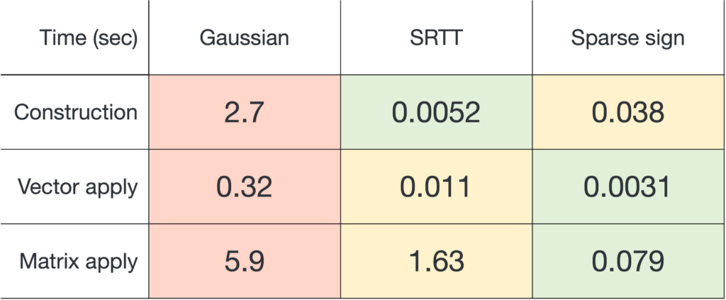
 and applying it to a matrix
  , sparse sign embeddings are 14× faster than SRTTs and 73× faster than Gaussian embeddings.
 for
for  and
and  using the MATLAB
  (equivalently,
  ) is shown as a dashed line.
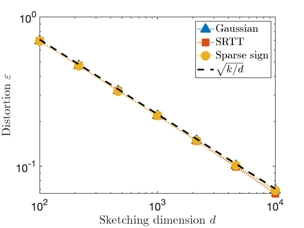
 is taken to be a matrix with independent standard Gaussian random values.
 is taken to be the
  is taken to be the
  identity matrix stacked onto a
  matrix of zeros.
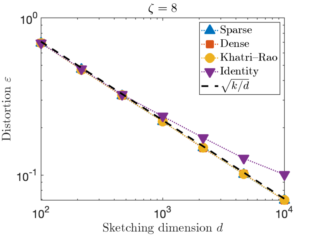
 . However, for the last test matrix “Identity”, we see the distortion begins to slightly exceed this predicted distortion for
  .
. , we can increase the value of the sparsity parameter
  . We recommend
 ![\[\zeta = \max \left( 8 , \left\lceil 2\sqrt{\frac{d}{k}} \right\rceil \right).\]](https://www.ethanepperly.com/wp-content/ql-cache/quicklatex.com-5f1ebe7695d9918399b0f97b628fcce1_l3.png "Rendered by QuickLaTeX.com")
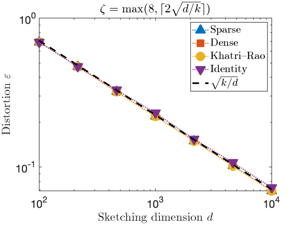
 can be necessary to achieve the optimal distortion.
![\[S = \frac{1}{\sqrt{\zeta}} \begin{bmatrix} s_1 & \cdots & s_n \end{bmatrix}.\]](https://www.ethanepperly.com/wp-content/ql-cache/quicklatex.com-4871e53b2bb59ad11946f2d1eafc66f7_l3.png "Rendered by QuickLaTeX.com")
 is an independent and randomly generated to contain exactly
  or
or  with 50/50 odds.
 to a smaller dimension
 ![\[(1-\varepsilon) \norm{x} \le \norm{Sx} \le (1+\varepsilon) \norm{x} \quad \text{for all }x \in \operatorname{col}(A).\]](https://www.ethanepperly.com/wp-content/ql-cache/quicklatex.com-41fd14292c1c85cd318dde801a75e1bd_l3.png "Rendered by QuickLaTeX.com")
![\[d = \frac{k}{\varepsilon^2} \quad \text{and} \quad \zeta = \max\left(8,\frac{2}{\varepsilon}\right).\]](https://www.ethanepperly.com/wp-content/ql-cache/quicklatex.com-ed85cec8dadffec7c7a3b4e099d6637d_l3.png "Rendered by QuickLaTeX.com")
 . The value
  has demonstrated deficiencies and should almost always be avoided (see below). The scaling
  is derived from the
 ![\[d = \mathcal{O} \left( \frac{k \log k}{\varepsilon^2} \right) \quad \text{and} \quad \zeta = \mathcal{O}\left( \frac{\log k}{\varepsilon} \right).\]](https://www.ethanepperly.com/wp-content/ql-cache/quicklatex.com-4fb6d0d60c85bc8a60d95bb0a19e63d6_l3.png "Rendered by QuickLaTeX.com")
 factor and the lack of explicit constants in the
  and can also be generated using a single line. The real challenge to generating sparse sign embeddings in MATLAB is the row indices, since each batch of
  sparse sign embedding with sparsity
  and weights
  . To apply
  and reweight them using the weights:
![\[b \in \real^n \longmapsto Sb = (w_1 b_{i_1},\ldots,w_db_{i_d}) \in \real^d.\]](https://www.ethanepperly.com/wp-content/ql-cache/quicklatex.com-712b97fc6f6efb9bf9a40dac2a652f5c_l3.png "Rendered by QuickLaTeX.com")
 for the hard “Identity” test matrix used above.
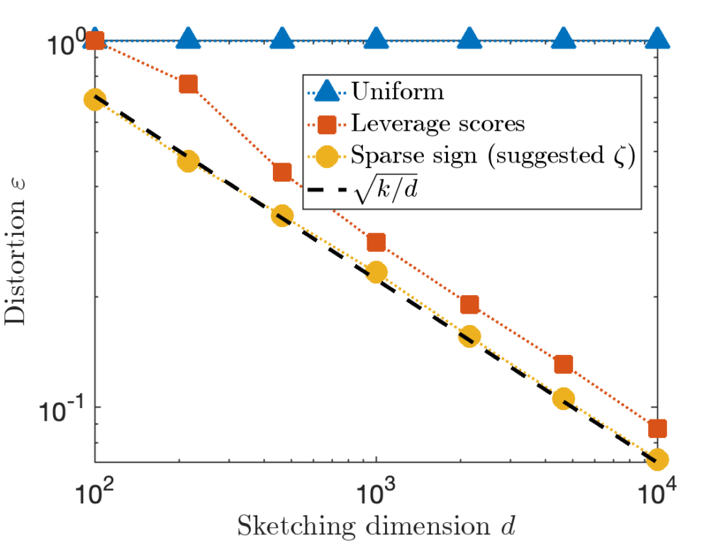
 for each row of
  cost, much higher than other types of sketches.
 , and compare the distortion of CountSketch to the sparse sign embedding with parameters
  :
: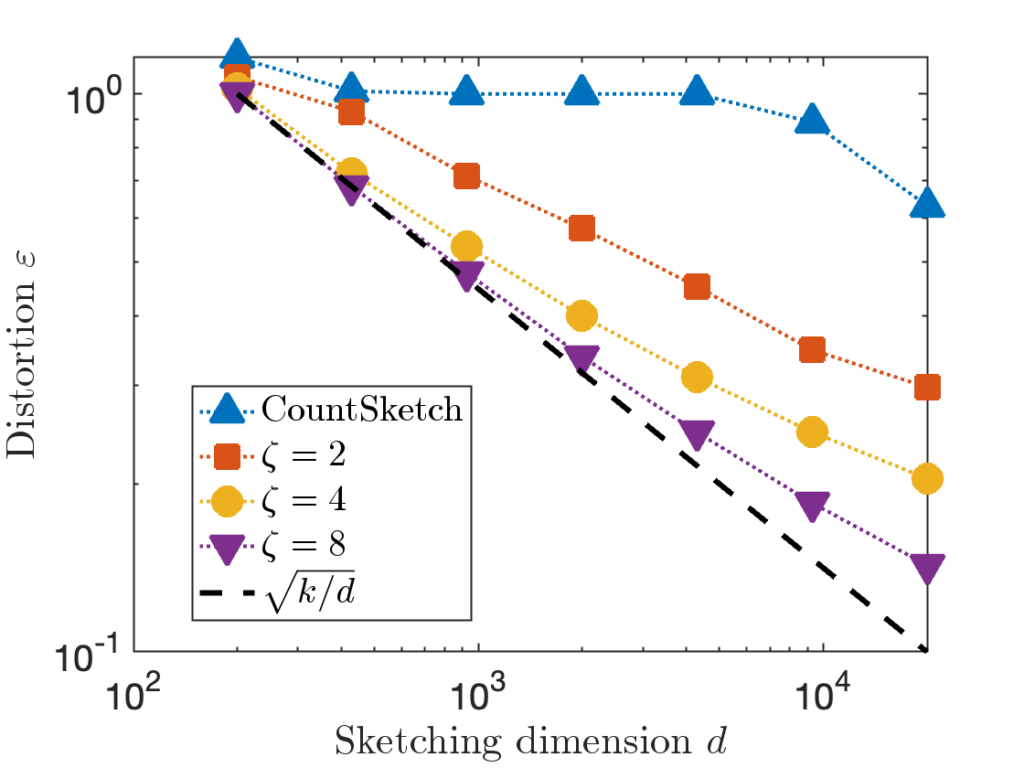
 , 20× higher than
  in order to achieve distortion
  (or perhaps
  ). This difference between
  for CountSketch and
  for other sketching matrices is a at the root of CountSketch’s woefully bad performance on some inputs.
 is an informal symbol meaning “proportional to”.
 . This is Theorem 16 in
  , where
  and
and  .
. is a CountSketch matrix with output dimension
  , then the distortion of
  with high probability.
![\[SA = \begin{bmatrix} s_1 & \cdots & s_k \end{bmatrix}\]](https://www.ethanepperly.com/wp-content/ql-cache/quicklatex.com-82c7ea0e5c52b6bd9bdb389f3d3f92d7_l3.png "Rendered by QuickLaTeX.com")
 has a single
  in a uniformly random location
  .
.
 are not all different from each other, say
  . Set
. Set  , where
  is the standard basis vector with
  and zeros elsewhere. Then,
  but
but  . Thus, for the distortion relation
 ![\[(1-\varepsilon) \norm{x} =(1-\varepsilon)\sqrt{2} \le 0 = \norm{(SA)x}\]](https://www.ethanepperly.com/wp-content/ql-cache/quicklatex.com-b08feebb30829a0e73b02188eba6f901_l3.png "Rendered by QuickLaTeX.com")
 . Thus,
 ![\[\prob \{ \varepsilon \ge 1 \} \ge \prob \{ j_1,\ldots,j_k \text{ are not distinct} \}.\]](https://www.ethanepperly.com/wp-content/ql-cache/quicklatex.com-12fa7b716b97c7e9482f4f6327bd4728_l3.png "Rendered by QuickLaTeX.com")
 pairs of people. Each pair of people has a
  chance of sharing a birthday, so the expected number of birthdays in a room of 23 people is
  . Since are 0.69 birthdays shared on average in a room of 23 people, it is perhaps less surprising that 23 is the critical number at which the chance of two people sharing a birthday exceeds 50%.
 and
and  in CountSketch have a
  pairs of indices, so the expected number of equal indices
  . Thus, we should anticipate
  is required to ensure that
 ![\[\prob \{ j_1,\ldots,j_k \text{ are not distinct} \} = 1 - \prob \{ j_1,\ldots,j_k \text{ are distinct} \}.\]](https://www.ethanepperly.com/wp-content/ql-cache/quicklatex.com-338a38501a565185b794f8ed03803c9a_l3.png "Rendered by QuickLaTeX.com")
 are all distinct, the probability
  are distinct is just the probability that
  values
 ![\[\prob\{ j_1,\ldots,j_i \text{ are distinct} \mid j_1,\ldots,j_{i-1} \text{ are distinct}\} = 1 - \frac{i-1}{d}.\]](https://www.ethanepperly.com/wp-content/ql-cache/quicklatex.com-b474f00c44e53b7c3c398d56121e1ac3_l3.png "Rendered by QuickLaTeX.com")
![\[\prob \{ j_1,\ldots,j_k \text{ are distinct} \} = \prod_{i=1}^k \left(1 - \frac{i-1}{d} \right).\]](https://www.ethanepperly.com/wp-content/ql-cache/quicklatex.com-7dd28281f8dbed8b3a1452a21e7410c8_l3.png "Rendered by QuickLaTeX.com")
 for every
  , obtaining
![\[\mathbb{P} \{ j_1,\ldots,j_k \text{ are distinct} \} \le \prod_{i=0}^{k-1} \exp\left(-\frac{i}{d}\right) = \exp \left( -\frac{1}{d}\sum_{i=0}^{k-1} i \right) = \exp\left(-\frac{k(k-1)}{2d}\right).\]](https://www.ethanepperly.com/wp-content/ql-cache/quicklatex.com-8d9d4c7d12af0fd89e53ca261c5df287_l3.png "Rendered by QuickLaTeX.com")
![\[\prob \{ \varepsilon \ge 1 \} \ge 1-\prob \{ j_1,\ldots,j_k \text{ are distinct} \\}\ge 1-\exp\left(-\frac{k(k-1)}{2d}\right).\]](https://www.ethanepperly.com/wp-content/ql-cache/quicklatex.com-144cfc73d778c4f9ed7442f5a6610e5e_l3.png "Rendered by QuickLaTeX.com")
![\[\prob\{\varepsilon \ge 1\} \ge \frac{1}{2} \quad \text{if} \quad d \le \frac{k(k-1)}{2\ln 2}.\]](https://www.ethanepperly.com/wp-content/ql-cache/quicklatex.com-e11567078a415b79b06a8e5e6f0b1600_l3.png "Rendered by QuickLaTeX.com")
 or perhaps a tall matrix
  . A sketching matrix is a
  matrix
  . When multiplied into a high-dimensional vector
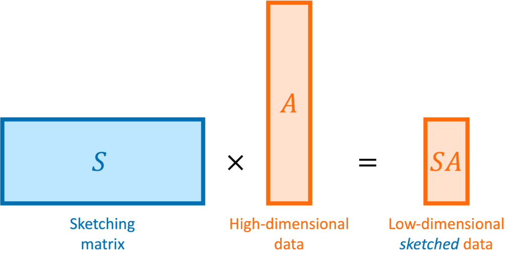
 be a collection of vectors. For
  , we require that
  :
: ![\[(1-\varepsilon) \norm{x}\le\norm{Sx}\le(1+\varepsilon)\norm{x} \]](https://www.ethanepperly.com/wp-content/ql-cache/quicklatex.com-735df49a45ff5d0bb27d478569004bdd_l3.png "Rendered by QuickLaTeX.com")
![\[\operatorname{col}(A) \coloneqq \{ Ax : x \in \real^k \}.\]](https://www.ethanepperly.com/wp-content/ql-cache/quicklatex.com-5ecde6b43df29caba14fd43682b4cc86_l3.png "Rendered by QuickLaTeX.com")
 with an output dimension of roughly
  . In particular, the sketching dimension
  in the column space of
  requires roughly
  operations, rather than the
  operations we would expect to multiply a
  is
is ![\[S = \sqrt{\frac{n}{d}} \cdot R \cdot F \cdot D.\]](https://www.ethanepperly.com/wp-content/ql-cache/quicklatex.com-92095cbf9c7d55273bd572a33debe415_l3.png "Rendered by QuickLaTeX.com")
 is a diagonal matrix whose entries are each a random
  (chosen independently with equal probability).
 is a fast trigonometric transform such as a fast
  is a selection matrix. To generate
  , let
, let  , selected without replacement.
  for every vector
  and the
  operations, a significant improvement over the
  , larger than for a Gaussian sketch.
![\[S = \frac{1}{\sqrt{\zeta}} \begin{bmatrix} s_1 & s_2 & \cdots & s_n \end{bmatrix}.\]](https://www.ethanepperly.com/wp-content/ql-cache/quicklatex.com-bb5806806e2e5900d4351c08befbd82e_l3.png "Rendered by QuickLaTeX.com")
 nonzero entries. The parameter
  in practice.
 or
or  operations) to apply to a vector, depending on parameter choices (see below). With a good sparse matrix library, sparse sign embeddings are often the fastest sketching matrix by a wide margin.
 random numbers, higher than SRTTs (roughly
  numbers).
  ; the theoretically sanctioned sketching dimension (at least according to existing theory) is larger than for a Gaussian sketch. In practice, we can often get away with using
  .
. operations. Therefore, sketching offers the promise of speeding up linear algebraic computations involving
 ![\[\operatorname*{minimize}_{x\in\real^k} \norm{Ax - b}. \]](https://www.ethanepperly.com/wp-content/ql-cache/quicklatex.com-07528304ce875f54aa1173062c5ec10a_l3.png "Rendered by QuickLaTeX.com")
 .
.
 . Applying
 ![\[\operatorname*{minimize}_{\hat{x}\in\real^k} \norm{(SA)\hat{x} - Sb}. \]](https://www.ethanepperly.com/wp-content/ql-cache/quicklatex.com-7110d3e9c1dd7e29793603a5bafdd201_l3.png "Rendered by QuickLaTeX.com")
 , first apply sketching to obtain
  and then apply an out-of-the-box clustering algorithms like
  denote the optimal least-squares solution and let
 ![\[\norm{A\hat{x} - b} \le \frac{1+\varepsilon}{1-\varepsilon} \norm{Ax - b}.\]](https://www.ethanepperly.com/wp-content/ql-cache/quicklatex.com-3d1d034bd8bf93f1c15e435a27a355ee_l3.png "Rendered by QuickLaTeX.com")
 , then this bound tells us that
 ![\[\norm{A\hat{x} - b} \le 2\norm{Ax_\star - b}. \]](https://www.ethanepperly.com/wp-content/ql-cache/quicklatex.com-588170743415f491f48ef2adc3d46628_l3.png "Rendered by QuickLaTeX.com")
 . For such applications, the bound (4) ensures that
  . Often, this means
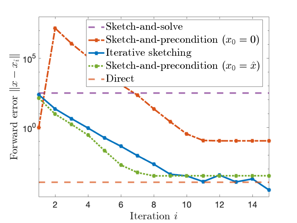
  , measuring how close
  and residual norm
  ). Then, we generate a sparse sign embedding of dimension
  ). Then, we compute the sketch-and-solve solution and, as reference, a “direct” solution by
  , close to direct method’s residual norm of
  . However, the forward error of sketch-and-solve is
  nine orders of magnitude larger than the direct method’s forward error of
  .
. , to decrease the distortion by a factor of ten requires increasing the sketching dimension
  that we hope will converge at a rapid rate to the true least-squares solution,
  , then
  .
.![\[SA = QR,\]](https://www.ethanepperly.com/wp-content/ql-cache/quicklatex.com-9edf84077821e9e0cd0c772b77024799_l3.png "Rendered by QuickLaTeX.com")
![\[A^\top A \approx (SA)^\top (SA) = R^\top Q^\top Q R = R^\top R.\]](https://www.ethanepperly.com/wp-content/ql-cache/quicklatex.com-90e14ee1172525fd795980cb3ef1a647_l3.png "Rendered by QuickLaTeX.com")
 .
.
![\[(A^\top A)x = A^\top b. \]](https://www.ethanepperly.com/wp-content/ql-cache/quicklatex.com-3f3c5265345a169d6633a759854510da_l3.png "Rendered by QuickLaTeX.com")
 in (5) and solving. The resulting solution is
![\[x_0 = R^{-1} (R^{-\top}(A^\top b)).\]](https://www.ethanepperly.com/wp-content/ql-cache/quicklatex.com-6b63093ea5c1d9714fb0deab43fc4dc3_l3.png "Rendered by QuickLaTeX.com")
 will typically not be a good solution to the least-squares problem (2), so we need to iterate. To do so, we’ll try and solve for the error
  . To derive an equation for the error, subtract
  from both sides of the normal equations (5), yielding
 ![\[(A^\top A)(x-x_0) = A^\top (b-Ax_0).\]](https://www.ethanepperly.com/wp-content/ql-cache/quicklatex.com-4f1ee993844dbcd8e397f27ccd1deefb_l3.png "Rendered by QuickLaTeX.com")
 :
: ![\[x\approx x_1 \coloneqq x_0 + R^{-\top}(R^{-1}(A^\top(b-Ax_0))).\]](https://www.ethanepperly.com/wp-content/ql-cache/quicklatex.com-0496d7e3c8bc117e658c57fc167081be_l3.png "Rendered by QuickLaTeX.com")
 , approximate
  , and obtain a new approximate solution
  . Continuing this process, we obtain an iteration
![\[x_{i+1} = x_i + R^{-\top}(R^{-1}(A^\top(b-Ax_i))).\]](https://www.ethanepperly.com/wp-content/ql-cache/quicklatex.com-f8db238fc978e6a8fc968fc5e387ec27_l3.png "Rendered by QuickLaTeX.com")
 at every iteration. Later,
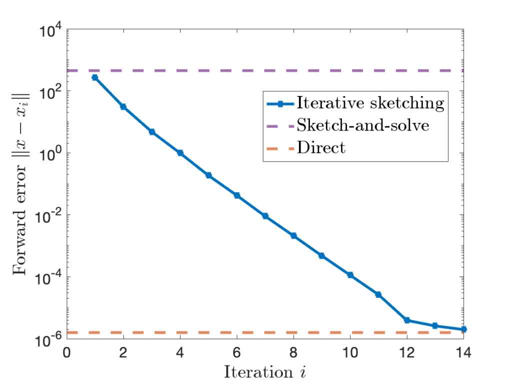
 to
to  by the iteration (6). If we run for enough iterations
  , the accuracy of the iterative sketching solution
  can be quite high.
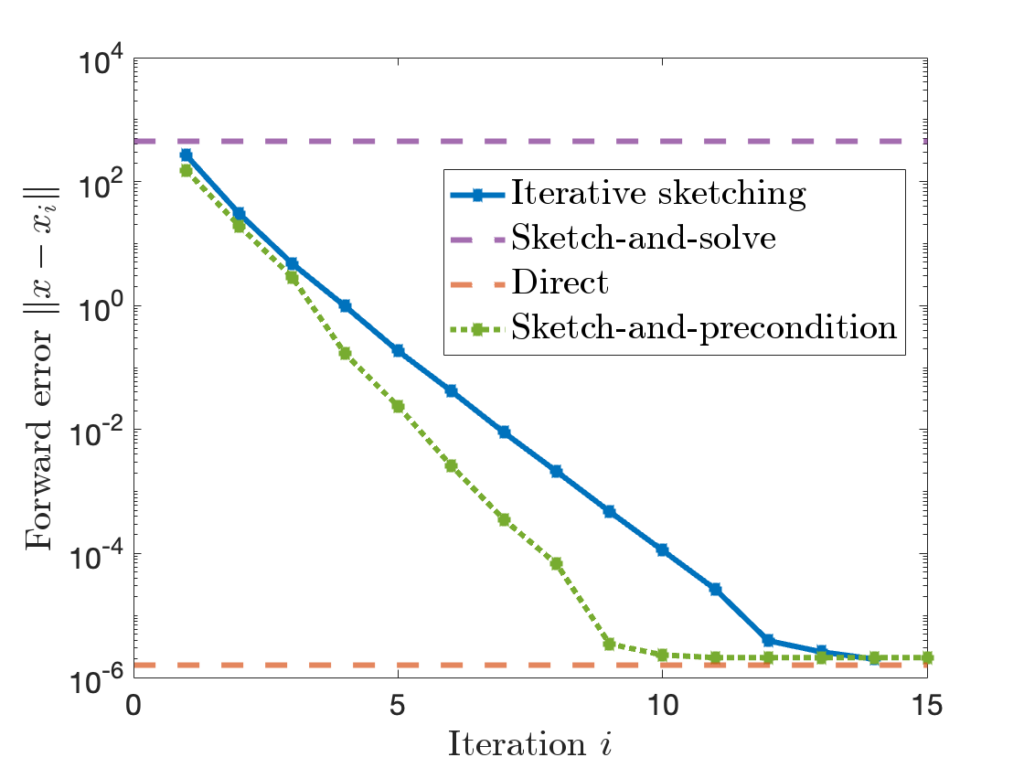
 is comparable to accuracy of a standard
  , sketch-and-precondition is not forward stable. The maximum achievable accuracy was worse than standard solvers by orders of magnitude! Maybe sketching doesn’t work after all?
 for sketch-and-precondition, then sketch-and-precondition appears to be forward stable in practice. No theoretical analysis supporting this finding is known at present.
 and residual
  .
.