Markov Musings 4: Should You Be Lazy?

August 16, 2023 by Ethan N. Epperly Leave a comment

This post is part of a series, Markov Musings, about the mathematical analysis of Markov chains. See here for the first post in the series.

In the previous post, we proved the following convergence results for a reversible Markov chain

$\chi^2\left(\rho^{(n)} \, \middle|\middle| \, \pi\right) \le \left( \max \{ \lambda_2, -\lambda_n \} \right)^{2n} \chi^2\left(\rho^{(0)} \, \middle|\middle| \, \pi\right).$

Here, $\rho^{(n)}$ denotes the distribution of the chain at time $n$ , $\pi$ denotes the stationary distribution, $\chi^2(\cdot \mid\mid \cdot)$ denotes the $\chi^2$ divergence, and $1 = \lambda_1 \ge \lambda_2 \ge \cdots \ge \lambda_m \ge -1$ denote the decreasingly ordered eigenvalues of the Markov transition matrix $P$ . To bound the rate of convergence to stationarity, we therefore must upper bound $\lambda_2$ and lower bound $\lambda_m$ .

Having to prove separate bounds for two eigenvalues is inconvenient. In the next post, we will develop tools to bound $\lambda_2$ . But what should we do about $\lambda_m?$ Fortunately, there is a trick.

It Pays to be Lazy

Call a Markov chain lazy if, at every step, the chain has at least a 50% chance of staying put. That is, $P_{ii} \ge 1/2$ for every $i$ .

Any Markov chain can be made into a lazy chain. At every step of the chain, flip a coin. If the coin is heads, perform a step of the Markov chain as normal, drawing the next step randomly according to the transition matrix $P$ . If the coin comes up tails, do nothing and stay put.

Algebraically, the lazy chain described in the previous paragraph corresponds to replacing the original transition matrix $P$ with the lazy transition matrix $P^{\rm lazy} \coloneqq (I+P)/2$ , where $I$ denotes the identity matrix. It is easy to see that the stationary distribution $\pi$ for $P$ is also a stationary distribution for $P^{\rm lazy}$ :

$\pi^\top P^{\rm lazy} = \frac{1}{2} \pi^\top P + \frac{1}{2} \pi^\top I = \frac{1}{2} \pi^\top + \frac{1}{2} \pi^\top = \pi^\top.$

The eigenvalues of the lazy transition matrix are

$\lambda_i^{\rm lazy} = \frac{1+\lambda_i}{2}.$

In particular, since all of the original eigenvalues $\lambda_i$ are $\ge -1$ , all of the eigenvalues of the lazy chain are $\ge 0$ . Thus, the smallest eigenvalue of $P^{\rm lazy}$ is always $\ge 0$ and thus, for the lazy chain, the convergence is controlled only by $\lambda_2^{\rm lazy}$ :

$\chi^2\left(\rho^{(n)} \, \middle|\middle| \, \pi\right) \le \left( \lambda_2^{\rm lazy} \right)^{2n} \chi^2\left(\rho^{(0)} \, \middle|\middle| \, \pi\right).$

Since it can be easier to establish bounds on the second eigenvalue than on both the second and last, it can be convenient—for theoretical purposes especially—to work with lazy chains, using the construction above to enforce laziness if necessary.

Should You be Lazy?

We’ve seen one theoretical argument for why it pays to use lazy Markov chains. But should we use lazy Markov chains in practice? The answer ultimately depends on how we want to use the Markov chain.

Here are two very different ways we could use a Markov chain:

One-shot sampling. Run the Markov chain once for a fixed number of steps $n$ , and use the result as an approximate sample from $\pi$ .

For this use case, it is important that the output is genuinely a sample from $\pi$ , and the possibility of large negative eigenvalues can significantly degrade the convergence. In the extreme case where $-1$ is an eigenvalue, the chain will fail to converge to stationarity at all. For this application, the lazy approach may make sense.

Averaging. Another way we can use a Markov chain is to compute the average of value of a function $f(x)$ over a random variable $x\sim\pi$ drawn from the stationary distribution:
$\expect_{x\sim \pi} [f(x)] = \sum_{i=1}^m f(i) \pi_i.$
To do this, we approximate this expectation by the time average $\hat{f}_N$ of the value of $f$ over the first $N$ values $x_0,x_1,\ldots,x_{N-1}$ of the chain
$\hat{f}_{N}\coloneqq \frac{1}{N}\sum_{n=0}^{N-1} f(x_i).$

As we shall see, this averaging process converges at an (asymptotically) slower rate for the lazy chain than the original chain. Therefore, for this application, we should typically just run the chain as-is, and not worry about making it lazy.

The Case Against Laziness

To see why being lazy hurts us for the averaging problem, we will use the Markov chain central limit theorem. As with many random averaging processes, we expect that in the limit of a large number of steps $N$ , the Markov chain average

$\hat{f}_N = \frac{1}{N}\sum_{n=0}^{N-1} f(x_i)$

will become approximately normally distributed. This is the content of the Markov chain central limit theorem (CLT):

Informal theorem (Markov chain central limit theorem). Let $x_0,x_1,x_2,\ldots$ denote the states of a Markov chain initialized in the stationary distribution $x_0\sim\pi$ . For a large number $N$ of steps, $\hat{f}_N$ is approximately normally distributed with mean $\expect_{x\sim \pi} [f(x)]$ and variance $\sigma^2/N$ where
(1) $\sigma^2 = \Var[f(x_0)] + 2\sum_{n=1}^\infty \Cov(f(x_0),f(x_n)).$

The Markov chain CLT shows that the variance of the Markov chain average $\hat{f}_N$ depends not only on the variance of $f$ in the stationary distribution, but also the covariance between $f(x_0)$ and later values $f(x_n)$ . The faster the covariance decreases, the smaller $\sigma^2$ will be and thus the smaller the error for the Markov chain average.

More formally, the Markov chain CLT is given by the following result:

Theorem (Markov chain central limit theorem). As $N\to\infty$ ,
$\frac{\hat{f}_N - \expect_{x \sim \pi} [f(x)]}{\sqrt{N}}$
converges in distribution to a normal random variable with mean zero and variance $\sigma^2$ , as defined in (1).

To compare the lazy and non-lazy chains, let’s compute the variance parameter $\sigma^2$ in the Markov chain CLT in terms of the eigenvalues of the chain. For the remainder of this post, let $f : \{1,\ldots,m\} \to \real$ be any function.

Step 1: Spectral Decomposition

Recall that, by the spectral theorem, the transition matrix $P$ has eigenvectors $\varphi_1,\varphi_2,\ldots,\varphi_m$ that are orthonormal in the $\pi$ -inner product

$\langle \varphi_i,\varphi_j \rangle = \expect_{x\sim \pi} [\varphi_i(x)\varphi_j(x)] = \begin{cases}1, & i = j, \\0, & i \ne j.\end{cases}$

As in the previous post, we think of vectors such as $\varphi_i \in \real^m$ as defining a function $\varphi_i : \{1,\ldots,m\} \to \real$ . Thus, we can expand the function $f$ using the eigenvectors

(2) $f = c_1 \varphi_1 + \cdots + c_m \varphi_m.$

The first eigenvector $\varphi_1 = \mathbf{1}$ is the vector of all ones (or, equivalently, the function that outputs $1$ for every output).

Step 2: Applying the Transition Matrix to a Function

The transition matrix $P$ is defined so that if the Markov chain has probability distribution $\sigma^\top$ at time $n$ , then the chain has distribution $\sigma^\top P$ at time $n+1$ . In other words, multiplying by $P$ on the right advances a distribution forward one step in time. This leads us to ask, what is the interpretation of multiplying a function by $P$ on the left. That is, is there an interpretation to the matrix–vector product $Pf$ ?

Indeed, there is such an interpretation: The $i$ th coordinate of $Pf$ is the expectation of $f(x_1)$ conditional on the chain starting at $x_0 = i$ :

$(Pf)(i) = \expect[f(x_1) \mid x_0 = i].$

Similarly,

(3) $(P^nf)(i) = \expect[f(x_n) \mid x_0 = i].$

There’s a straightforward proof of this fact. Let $\delta_i^\top$ denote a probability distribution which places 100% of the probability mass on the single site $i$ . The $i$ th entry of $P^n f$ is

$(P^n f)(i) = \delta_i^\top (P^n f) = (\delta_i^\top P^n) f.$

We know that $\rho^{(n)} = \delta_i^\top P^n$ is the state of the Markov chain after $n$ steps when initialized in the initial distribution $\rho^{(n)} = \delta_i$ . Thus,

$(P^n f)(i) = (\rho^{(n)})^\top f = \sum_{i=1}^m \rho^{(n)}_i f(i) = \expect[f(x_n) \mid x_0=i].$

This proves the formula (3).

Step 3: Computing the Covariance

With the help of the formula for $P^nf$ and the spectral decomposition of $f$ , we are ready to compute the covariances appearing in (1).Let $x_0 \sim \pi$ . Then

(4) $\Cov (f(x_0),f(x_n)) = \expect[f(x_0)f(x_n)] - \expect[f(x_0)]\expect[f(x_n)].$

Let’s first compute $\expect[f(x_0)]$ and $\expect[f(x_n)]$ . Since $\varphi_1 = \mathbf{1}$ is the vector/function of all ones, we have

$\expect[f(x_0)] = \expect[f(x_0) \cdot 1] = \expect[f(x_0) \varphi_1(x_0)] = \langle f, \varphi_1\rangle = c_1.$

For the last equality, we use the spectral decomposition (2) along with the orthonormality of the eigenvectors $\varphi_i$ .

Since we assume the chain is initialized in the stationary distribution $x_0 \sim \pi$ , it remains in stationarity at time $n$ , $x_n \sim \pi$ , so we have $\expect[f(x_n)] = \expect[f(x_0)] = c_1$ .

Now, let’s compute $\expect[f(x_0)f(x_n)]$ . Use the law of total expectation to write

$\begin{align*}\expect[f(x_0)f(x_n)] &= \sum_{i=1}^m \expect[f(x_0) f(x_n) \mid x_0 = i] \prob\{x_0 = i\} \\&= \sum_{i=1}^m f(i) \expect[f(x_n) \mid x_0 = i] \pi_i.\end{align*}$

Now, invoke (3) and the definition of the $\pi$ -inner product to write

$\expect[f(x_0)f(x_n)] = \sum_{i=1}^m f(i) (P^n f)(i) \pi_i = \langle f, P^n f\rangle.$

Finally, using the spectral decomposition, we obtain

$\expect[f(x_0)f(x_n)] = \left\langle \sum_{i=1}^m c_i \varphi_i,\sum_{i=1}^m c_i P^n\varphi_i \right\rangle = \left\langle \sum_{i=1}^m c_i \varphi_i,\sum_{i=1}^m c_i \lambda_i^n \varphi_i \right\rangle = \sum_{i=1}^m \lambda_i^n \, c_i^2.$

Combining this formula with our earlier observation that $\expect[f(x_0)] = \expect[f(x_n)] = c_1$ and plugging into (4), we obtain

(5) $\Cov(f(x_0),f(x_n)) = \sum_{i=1}^m \lambda_i^n \, c_i^2 - c_1^2 = \sum_{i=2}^m \lambda_i^n c_i^2.$

For the second equality, we use that the largest eigenvalue is $\lambda_1 = 1$ , so $c_1$ entirely drops out of the covariance.

Step 4: Wrapping it Up

With the formula (5) for the covariance in hand, we are ready to evaluate the $\sigma^2$ variance parameter in the Markov chain CLT. First, note that the variance is

$\Var[f(x_0)] = \Cov(f(x_0),f(x_0)) = \sum_{i=2}^m \lambda_i^0 c_i^2 = \sum_{i=2}^m c_i^2.$

Therefore, combining this formula for the variance and the formula (5) for the covariance, we obtain

$\begin{align*}\sigma^2 &= \Var[f(x_0)] + 2\sum_{n=1}^\infty \Cov(f(x_0),f(x_n)) \\&= \sum_{i=2}^m c_i^2 + 2\sum_{n=1}^\infty \sum_{i=2}^m \lambda_i^n \, c_i^2 \\&= -\sum_{i=2}^m c_i^2 + 2\sum_{i=2}^m \left(\sum_{n=0}^\infty \lambda_i^n\right)c_i^2 .\end{align*}$

Now, apply the formula for the sum of an infinite geometric series to obtain

(6) $\sigma^2 = -\sum_{i=2}^m c_i^2 + 2\sum_{i=2}^m \frac{1}{1-\lambda_i} c_i^2 = \sum_{i=2}^m \left(\frac{2}{1-\lambda_i}-1\right)c_i^2 = \sum_{i=2}^m \frac{1+\lambda_i}{1-\lambda_i} c_i^2.$

Conclusion: Laziness is (Asymptotically) Bad for Averaging

Before we get to the conclusions, let’s summarize where we are. We are seeking to use Markov chain average

$\hat{f}_N = \frac{1}{N} \sum_{i=0}^{N-1} f(x_n)$

as an approximation to the stationary mean $\expect_{x \sim \pi} [f(x)]$ . The Markov chain central limit theorem shows that, for a large number of steps $N$ , the error $\hat{f}_N - \expect_{x\sim\pi}[f(x)]$ is approximately normally distributioned with mean zero and variance $\sigma^2/N$ . So to obtain accurate estimates, we want $\sigma^2$ to be as small as possible.

After some work, we were able to derive a formula (6) for $\sigma^2$ in terms of the eigenvalues $\lambda_1,\ldots,\lambda_m$ of the transition matrix $P$ . The formula for $\sigma^2$ for the lazy chain is identical, except with each eigenvalue replaced by $(\lambda_i+1)/2$ . Thus, we have

$\begin{align*}\sigma^2_{\rm nonlazy} &= \sum_{i=2}^m \frac{1+\lambda_i}{1-\lambda_i} c_i^2, \\\sigma^2_{\rm lazy} &= \sum_{i=2}^m \frac{3+\lambda_i}{1-\lambda_i} c_i^2.\end{align*}$

From these formulas, it is clear that the lazy Markov chain has a larger $\sigma^2$ parameter and is thus less accurate than the non-lazy Markov chain, no matter what the eigenvalues are.

To compare the non-lazy and lazy chains in another way, consider the plot below. The blue solid line shows the amplification factor $(1-\lambda_i)/(1+\lambda_i)$ of an eigenvalue $\lambda_i$ , which represents amount by which the squared coefficient $c_i^2$ is scaled by in $\sigma^2$ . In the red-dashed line, we see the corresponding amplification factor $(1-\lambda_i^{\rm lazy})/(1+\lambda^{\rm lazy}_i)$ for the corresponding eigenvalue $\lambda^{\rm lazy}_i = (\lambda_i+1)/2$ of the lazy chain. We see that at every $\lambda$ value, the lazy chain has a higher amplification factor than the original chain.

Remember that our original motivation for using the lazy chain was to remove the possibility of slow convergence of the chain to stationarity because of negative eigenvalues. But for the averaging application, negative eigenvalues are great. The process of Markov chain averaging shrinks the influence of negative eigenvalues on $\sigma^2$ , whereas positive eigenvalues are amplified. For the averaging application, negative eigenvalues for the chain are a feature, not a bug.

Moral of the Story

Much of Markov chain theory, particularly in theoretical parts of computer science, mathematics, and machine learning, is centered around proving convergence to stationarity. Negative eigenvalues are a genuine obstruction to convergence to stationarity, and using the lazy chain in practice may be a sensible idea if one truly needs a sample from the stationary distribution in a given application.

But one-shot sampling is not the only or even the most common uses for Markov chains in computational practice. For other applications, such as averaging, the negative eigenvalues are actually a help. Using the lazy chain in practice for these problems would be a poor idea.

To me, the broader lesson in this story is that, as applied mathematicians, it can be inadvisable to become too fixated on one particular mathematical benchmark for designing and analyzing algorithms. Proving rapid convergence to stationarity with respect to the total variation distance is one nice way to analyze Markov chains. But it isn’t the only way, and chains not possessing this property because of large negative eigenvalues may actually be better in practice for some problems. Ultimately, applied mathematics should, at least in part, be guided by applications, and paying attention to how algorithms are used in practice should inform how we build and evaluate new ones.

Markov Musings 3: Spectral Theory

July 13, 2023 by Ethan N. Epperly 1 Comment

This post is part of a series, Markov Musings, about the mathematical analysis of Markov chains. See here for the first post in the series.

In the previous two posts, we proved the fundamental theorem of Markov chains using couplings and discussed the use of couplings to bound the mixing time, the time required for the chain to mix to near-stationarity.

In this post, we will continue this discussion by discussing spectral methods for understanding the convergence of Markov chains.

Mathematical Setting

In this post, we will study a reversible Markov chain on $\{1,\ldots,m\}$ with transition probability matrix $P \in \real^{m\times m}$ and stationary distribution $\pi$ . Our goal will be to use the eigenvalues and eigenvectors of the matrix $P$ to understand the properties of the Markov chain.

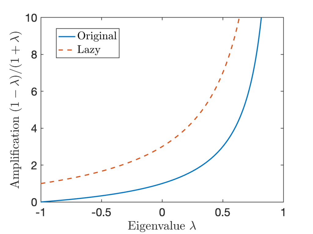
Throughout our discussion, it will be helpful to treat vectors $f\in\real^m$ and functions $f:\{1,\ldots,m\}\to \real$ as being one and the same, and we will use both $f_i$ and $f(i)$ to denote the $i$ th entry of the vector $f$ (aka the evaluation of the function $f$ at $i$ ). By adopting this perspective, a vector is not merely a list of $m$ numbers, but instead labels each state $i=1,2,\ldots,m$ with a numeric value.

Given a function/vector $f$ , we let $\expect[f]$ denote the expected value of $f(X)$ where $X$ is drawn from $\pi$ :

$\expect[f] \coloneqq \expect_{X \sim \pi} [f(X)] = \sum_{i=1}^m \pi_i f(i).$

The variance is defined similarly:

$\Var(f) \coloneqq \expect [(f - \expect[f])^2] = \sum_{i=1}^m (f(i) - \expect[f])^2 \pi_i.$

As a final piece of notation, we let $\delta_i$ denote a probability distribution which assigns 100% probability to outcome $i$ .

Spectral Theory

The eigenvalues and eigenvectors of general square matrices are ill-behaved creatures. Indeed, a general $m\times m$ matrix with real entries can have complex-valued eigenvalues and fail to possess a full suite of $m$ linearly independent eigenvectors. The situation is dramatically better for symmetric matrices which obey the spectral theorem:

Theorem (spectral theorem for real symmetric matrices). An $m\times m$ real symmetric matrix $A$ (i.e., one satisfying $A^\top=A$ ) has $m$ real eigenvalues $\lambda_1,\ldots,\lambda_m$ and $m$ orthonormal eigenvectors $u_1,\ldots,u_m$ .

Unfortunately for us, the transition matrix $P$ for a reversible Markov chain is not always symmetric. But despite this, there’s a surprise: $P$ always has real eigenvalues. This leads us to ask:

Why does are the eigenvalues of the transition matrix $P$ real?

To answer this question, we will need to develop and a more general version of the spectral theorem and use our standing assumption that the Markov chain is reversible.

The Transpose

In our quest to develop a general version of the spectral theorem, we look more deeply into the hypothesis of the theorem, namely that $A$ is equal to its transpose $A^\top$ . Let’s first ask: What does the transpose $A^\top$ mean?

Recall that $\real^m$ is equipped with the standard inner product, sometimes called the Euclidean or dot product. We denote this product by $(\cdot,\cdot)$ and it is defined as

$(f,g) \coloneqq f^\top g = \sum_{i=1}^m f(i) g(i).$

We can think of the standard inner product as defining the amount of the vector $f$ that points in the direction of $g$ .

The transpose of a matrix $A$ is closely related to the standard inner product. Specifically, $A^\top$ is the (unique) matrix satisfying the adjoint property:

$(f,Ag) = (A^\top f, g)\quad \text{for every }f,g\in\real^m.$

So the amount of $f$ in the direction of $Ag$ is the same as the amount of $A^\top f$ in the direction of $g$ .

The Adjoint and the General Spectral Theorem

Since the transpose is intimately related to the standard inner product on $\real^m$ , it is natural to wonder if non-standard inner products on $\real^m$ give rise to non-standard versions of the transpose. This idea proves to be true.

Definition (adjoint). Let $[\cdot,\cdot]$ be any inner product on $\real^m$ and let $A$ be an $m\times m$ matrix. The adjoint of $A$ with respect to the inner product $[\cdot,\cdot]$ is the (unique) matrix $A^*$ such that
$[f,Ag]=[A^*f,g]\quad\text{for every }f,g\in\real^m.$
A matrix $A$ is self-adjoint if it equals its own adjoint, $A=A^*$ .

The spectral theorem naturally extends to the more abstract setting of adjoints with respect to non-standard inner products:

Theorem (general spectral theorem). Let $A$ be an $m\times m$ matrix which is set-adjoint with respect to an inner product $[\cdot,\cdot]$ . Then $A$ has $m$ real eigenvalues $\lambda_1,\ldots,\lambda_m$ and $m$ eigenvectors $u_1,\ldots,u_m$ which are $[\cdot,\cdot]$ –orthonormal:
$[u_i,u_j]=\begin{cases}1, & i=j, \\0,& i\ne j.\end{cases}$

Reversibility and Self-Adjointness

The general spectral theorem offers us a path to understand our observation from above that the eigenvalues of $P$ are always real. Namely, we ask:

Is there an inner product under which $P$ is self-adjoint?

Fortunately, the answer is yes. Define the $\pi$ -inner product

$\langle f, g \rangle \coloneqq \expect[f\cdot g] = \sum_{i=1}^m f(i)g(i) \pi_i.$

This inner product is very natural. If $f$ and $g$ are mean-zero ( $\expect[f] = \expect[g] = 0$ ), it reports the covariance of $f(x)$ and $g(x)$ where $x \sim \pi$ is drawn from $\pi$ .

Let us compute the adjoint of the transition matrix $P$ in the $\pi$ -inner product $\langle \cdot,\cdot \rangle$ :

$\begin{align*}\langle f, Pg \rangle&= \sum_{i=1}^m f(i) \left(\sum_{j=1}^m P_{ij} g(i) \right)\pi_i= \sum_{i,j=1}^m f(i) g(j) \pi_iP_{ij} .\end{align*}$

Recall that we have assumed our Markov chain is reversible. Thus, the detailed balance condition

$\pi_i P_{ij} = \pi_j P_{ji} \quad \text{for } i,j=1,2,\ldots,m$

implies that

$\langle f, Pg \rangle= \sum_{i,j=1}^m f(i) g(j) \pi_jP_{ji} = \sum_{j=1}^m \left( \sum_{i=1}^m f(i) P_{ij} \right) g(j) \pi_j = \langle Pf, g\rangle.$

Thus, we conclude that $P$ is self-adjoint.

We cannot emphasize enough that the reversibility assumption is crucial to ensure that $P$ is self-adjoint. In fact,

Theorem (reversibility and self-adjointness). The transition matrix of a general Markov chain with stationary distribution $\pi$ is self-adjoint in the $\pi$ -inner product if and only if the chain is reversible.

Spectral Theorem for Markov Chains

Since $P$ is self-adjoint in the $\pi$ -inner product, the general spectral theorem implies the following

Corollary (spectral theorem for reversible Markov chain). The reversible Markov transition matrix $P$ has $m$ real eigenvalues $\lambda_1 \ge \cdots \ge \lambda_m$ associated with eigenvectors $\varphi_1,\ldots,\varphi_m$ which are orthonormal in the $\pi$ -inner product:
$\langle\varphi_i,\varphi_j\rangle=\begin{cases}1, &i=j\\0,& i\ne j.\end{cases}$

Since $P$ is a reversible Markov transition matrix—not just any self-adjoint matrix—the eigenvalues of $P$ satisfy additional properties:

Bounded. All of the eigenvalues of $P$ lie between $-1$ and $1$ .¹
Eigenvalue 1. $\lambda_1 = 1$ is an eigenvalue of $P$ with eigenvector $\varphi_1 = \mathbf{1}$ , where $\mathbf{1}$ is a vector of all one’s.

For a primitive chain, we can also have the property:

Contractive. For a primitive chain, all eigenvalues other than $\lambda_1$ have magnitude $< 1$ .²

Distance Between Probability Distributions Redux

In the previous post, we used the total variation distance to compare probability distributions:

Definition (total variation distance). The total variation distance between probability distributions $\sigma$ and $\pi$ is
$\norm{\sigma - \pi}_{\rm TV} = \max_{A \subseteq \{1,\ldots,m\}} |\sigma(A) - \pi(A)| = \frac{1}{2} \sum_{i=1}^m |\sigma_i - \pi_i|.$

The total variation distance is an “ $\ell_1$ “ way of comparing two probability distributions since it can be computed by adding the absolute difference between the probabilities $\sigma_i$ and $\pi_i$ of each outcome. Spectral theory plays more nicely with an “ $\ell_2$ ” way of comparing probability distributions, which we develop now.

Densities

Given two probability densities $\sigma$ and $\pi$ , the density of $\sigma$ with respect to $\pi$ is the function³ $h = d\sigma/d\pi$ given by

$h(i) = \frac{d\sigma}{d\pi}(i) = \frac{\sigma_i}{\pi_i} \quad \text{for } i=1,2,\ldots,m.$

The density $h = d\sigma/d\pi$ satisfies the property that

(1) $\expect_{X \sim \sigma} [g(X)] = \expect_{Y \sim \pi}[g(Y)h(Y)] = \sum_{i=1}^m g(i)h(i) \pi_i.$

To see why we call $h = d\sigma/d\pi$ a density, it may be helpful to appeal to continuous probability for a moment. If $0\le X \le 1$ is a random variable with distribution $\sigma$ , the probability density function of $\sigma$ (with respect to the uniform distribution $\mathrm{Unif}[0,1]$ ) is a function $h$ such that

$\expect_{X \sim \sigma} [g(X)] = \expect_{Y\sim \mathrm{Unif}[0,1]} [g(Y)h(Y)] = \int_0^1 g(x) h(x) \, dx.$

The formula for the continuous case is exactly the same as the finite case (1) with sums $\sum_{i=1}^m (\cdots) \pi_i$ replaced with integrals $\int_0^1 (\cdots) \, dx$ .

The Chi-Squared Divergence

We are now ready to introduce our “ $\ell_2$ ” way of comparing probability distributions.

Definition ( $\chi^2$ -divergence). The $\chi^2$ -divergence of $\sigma$ with respect to $\pi$ is the variance of the density function:
$\chi^2(\sigma \mid\mid \pi) \coloneqq \Var \left(\frac{d\sigma}{d\pi} \right) = \expect \left[\left( \frac{d\sigma}{d\pi} - 1 \right)^2\right] = \expect \left[\left(\frac{d\sigma}{d\pi}\right)^2\right] - 1.$

To see the last equality is a valid formula for $\chi^2(\sigma\mid\mid\pi) \coloneqq \Var(d\sigma/d\pi)$ , note that

(2) $\expect\left[\frac{d\sigma}{d\pi}\right] = \sum_{i=1}^m \frac{d\sigma}{d\pi}(i) \pi_i = \sum_{i=1}^m \frac{\sigma_i}{\pi_i} \pi_i = \sum_{i=1}^m \sigma_i = 1.$

Relations Between Distance Measures

The $\chi^2$ divergence always gives an upper bound on the total variation distance. Indeed, first note that we can express the total variation distance as

$\norm{\sigma - \pi}_{\rm TV} = \frac{1}{2} \expect \left[ \left| \frac{d\sigma}{d\pi} - 1 \right| \right].$

Thus, using Lyapunov’s inequality, we conclude

(3) $\norm{\sigma - \pi}_{\rm TV} = \frac{1}{2} \expect \left[ \left| \frac{d\sigma}{d\pi} - 1 \right| \right] \le \frac{1}{2} \left(\expect \left[ \left( \frac{d\sigma}{d\pi} - 1 \right)^2 \right]\right)^{1/2} = \frac{1}{2} \sqrt{\chi^2(\sigma \mid\mid \pi)}.$

Markov Chain Convergence by Eigenvalues

Now, we prove a quantitative version of the fundamental theorem of Markov chains (for reversible processes) using spectral theory and eigenvalues:⁴

Theorem (Markov chain convergence by eigenvalues). Let $\rho^{(0)},\rho^{(1)},\rho^{(2)},\ldots$ denote the distributions of the Markov chain at times $0,1,2,\ldots$ . Then
$\chi^2\left(\rho^{(n)} \, \middle|\middle| \, \pi\right) \le \left( \max \{ \lambda_2, -\lambda_n \} \right)^{2n} \chi^2\left(\rho^{(0)} \, \middle|\middle| \, \pi\right).$

This raises a natural question: How large can the initial $\chi^2$ divergence between $\rho^{(0)}$ and $\pi$ be? This is answered by the next result.

Proposition (Initial distance to stationarity). For any $i \in \{1,\ldots,m\}$ ,
(4) $\chi^2(\delta_i \mid\mid \pi) \le \frac{1}{\pi_i}.$
For any initial distribution $\rho^{(0)}$ , we have
(5) $\chi^2\left( \rho^{(0)} \, \middle|\middle| \, \pi \right) \le \frac{1}{\min_{1\le i\le m} \pi_i}$

The condition (4) is a direct computation

$\chi^2(\delta_i \mid\mid \pi) = \Var(d\delta_i/d\pi) \le \expect[(d\delta_i/d\pi)^2] = 1/\pi_i.$

For (5), observe that $\chi^2(\rho^{(0)} \mid\mid \pi)$ is a convex function of the initial distribution $\rho^{(0)}$ . Therefore, its maximal value over the convex set of all probability distribution is maximized at an extreme point $\rho^{(0)} = \delta_i$ for some $i$ . Consequently, (5) follows directly from (4).

Using the previous two results and equation (3), we immediately obtain the following:

Corollary (Mixing time). When initialized from a distribution $\rho^{(0)}$ , the chain mixes to $\varepsilon$ -total variation distance to stationarity
$\norm{\rho^{(n)} - \pi}_{\rm TV} \le \varepsilon$
after
(6) $n = \left\lceil \frac{1}{\log(\max\{\lambda_2,-\lambda_n\})}\log \left( \frac{1}{2\varepsilon \min_{1\le i \le m}\sqrt{\pi_i}} \right) \right\rceil \text{ steps}.$

Indeed,

$\begin{align*}\norm{\rho^{(n)} - \pi}_{\rm TV} &\le \frac{1}{2} \sqrt{\chi^2(\rho^{(n)} \mid\mid \pi)} \\&\le \frac{1}{2} (\max\{\lambda_2,-\lambda_n\})^n \sqrt{\chi^2(\rho^{(0)} \mid\mid \pi)} \\&\le \frac{(\max\{\lambda_2,-\lambda_n\})^n}{2\min_{1\le i \le m} \sqrt{\pi_i}}.\end{align*}$

Equating the left-hand side with $\varepsilon$ and rearranging gives (6).

Proof of Markov Chain Convergence Theorem

We conclude with a proof of the Markov chain convergence result.

Recurrence for Densities

Our first task is to derive a recurrence for the densities $d\rho^{(n)}/d\pi$ . To do this, we use the recurrence for the probability distribution:

$\rho^{(n+1)}_j = \sum_{i=1}^m \rho_i^{(n)} P_{ij}.$

Thus,

$\left( \frac{d\rho^{(n+1)}}{d\pi}\right)_j = \frac{\rho_j^{(n+1)}}{\pi_j} = \frac{\sum_{i=1}^m \rho^{(n)}_i P_{ij}}{\pi_j}= \sum_{i=1}^m \rho^{(n)}_i\frac{P_{ij}}{\pi_j}.$

We now invoke the detailed balance $P_{ij}/\pi_j = P_{ji} / \pi_i$ , which implies

$\left( \frac{d\rho^{(n+1)}}{d\pi}\right)_j = \sum_{i=1}^m\rho^{(n)}_i \frac{P_{ji}}{\pi_i} = \sum_{i=1}^m P_{ji} \frac{\rho^{(n)}_i}{\pi_i} = \left( P \frac{d \rho^{(n)}}{d\pi} \right)_j.$

The product $P(d\rho^{(n)}/d\pi)$ is an ordinary matrix–vector product. Thus, we have shown

(7) $\frac{d\rho^{(n+1)}}{d\pi} = P \frac{d\rho^{(n)}}{d\pi} \quad \text{for } n =0,1,\ldots.$

Spectral Decomposition

Now that we have a recurrence for the densities $d\rho^{(n)}/d\pi$ , we can understand how the densities change in time. Expand the initial density in eigenvectors of $P$ :

$\frac{d\rho^{(0)}}{d\pi} = c_1 \mathbf{1} + c_2 \varphi_2 + \cdots + c_m \varphi_m.$

As we verified above in (1), we have $\expect[d\rho^{(0)}/d\pi] = 1$ . Thus, we conclude $c_1 = 1$ . Since the $\varphi_j$ are eigenvectors of $P$ with eigenvalues $\lambda_j$ , the recurrence (7) implies

$\frac{d\rho^{(n)}}{d\pi} = \mathbf{1} + c_2 \lambda_2^n \varphi_2 + \cdots + c_m \lambda_m^n \varphi_m.$

Conclusion

Finally, we compute

$\chi^2(\rho^{(n)} \mid\mid \pi) = \sum_{i=2}^m c_i^2 \lambda_i^{2n} \le (\max \{ \lambda_2, -\lambda_m \})^{2n} \sum_{i=2}^m c_i^2 = (\max \{ \lambda_2, -\lambda_m \})^{2n} \chi^2(\rho^{(0)} \mid\mid \pi).$

The theorem is proven.

Markov Musings 2: Couplings

July 5, 2023 by Ethan N. Epperly Leave a comment

This post is part of a series, Markov Musings, about the mathematical analysis of Markov chains. See here for the first post in the series.

In the last post, we saw a proof of the fundamental theorem of Markov chains using the method of couplings. In this post, we will use couplings to provide quantitative bounds on the rate of Markov chain convergence.

Mixing Time

Let us begin where the last post ended by recalling some facts about the mixing time of a Markov chain. Consider a Markov chain $x_0,x_1,x_2,\ldots$ with stationary distribution $\pi$ . Recall that the mixing time is

$\tau_{\rm mix} \coloneqq \min \left\{ n \ge 1 : \max_{\rho^{(0)}} \norm{\rho^{(n)} - \pi}_{\rm TV} \le \frac{1}{2e} \right\}.$

Here, $\rho^{(n)}$ denotes the distribution of the state $x_n$ of the chain at time $n$ and $\norm{\cdot}_{\rm TV}$ is the total variation distance. For more on the total variation distance, see the previous post.

At the end of last post, we saw the following theorem, showing that the mixing time controls the rate of Markov chain convergence.

Theorem (mixing time as convergence rate). For any starting distribution $\rho^{(0)}$ ,
$\norm{\rho^{(n)} - \pi}_{\rm TV} \le e^{-\lfloor n / \tau_{\rm mix}\rfloor}.$
Consequently, if $n\ge \tau_{\rm mix}\cdot \lceil \log(1/\epsilon)\rceil$ , then $\norm{\rho^{(n)} - \pi}_{\rm TV} \le \varepsilon$ .

This result motivates us to develop techniques to bound the mixing time $\tau_{\rm mix}$ .

Couplings and Convergence

In the previous post, we made essential use of couplings of probability distributions. In this post, we will extend this notion by using couplings of entire Markov chains.

Definition (coupling of Markov chains). A coupling of Markov chains with transition matrix $P$ are two processes $x_0,x_1,x_2,\ldots$ and $y_0,y_1,y_2,\ldots$ such that (A) each process is individually a Markov chain with transition matrix $P$ : In particular,
$\prob\{x_{n+1} = j \mid x_n = i \} = \prob\{y_{n+1} = j \mid y_n = i \} = P_{ij}$
and (B) if $x_n = y_n$ , then $x_{n+1} = y_{n+1}$ .

A coupling of Markov chains thus consists of a pair of Markov chains which become glued together should they ever touch.

There are several ways we can use couplings to bound the mixing time of Markov chains. Here is one way. Let $x_0,x_1,x_2,\ldots$ and $y_0,y_1,y_2,\ldots$ be a coupling of Markov chains for which $x_0$ is initialized in some initial distribution $x_0 \sim \rho^{(0)}$ and $y_0$ is initialized in the stationary distribution $y_0 \sim \pi$ . Let $\tau_{\rho^{(0)}}$ be the time at which $x$ and $y$ meet:

$\tau_{\rho^{(0)}} \coloneqq \min\{ n \ge 0 : x_n = y_n\}.$

The following theorem shows that the tails of the random variable $\tau$ control the convergence of the Markov chain $x_0,x_1,x_2,\ldots$ to stationarity.

Theorem (convergence from couplings). Then $\norm{\rho^{(n)} - \pi}_{\rm TV} \le \prob\{\tau_{\rho^{(0)}} > n\}$ .

This result is an immediate application of the coupling lemma from last post. Using this bound, we can bound the mixing time

Corollary (mixing time from couplings). $\tau_{\rm mix} \le 2e \max_{\rho^{(0)}} \expect[\tau_{\rho^{(0)}}]$ .

The maximum is taken over all initial distributions $\rho^{(0)}$ .

Indeed, by the above theorem and Markov’s inequality,¹

$\norm{\rho^{(n)} - \pi}_{\rm TV} \le \prob\{\tau_{\rho^{(0)}} > n\}\le \frac{\expect[\tau_{\rho^{(0)}}]}{n}.$

Take a maximum over initial distribution $\rho^{(0)}$ and set $n \coloneqq \tau_{\rm mix}$ . Then the left-hand side is at most $1/2e$ , so

$\frac{1}{2e} \le \max_{\rho^{(0)}}\norm{\rho^{(\tau_{\rm mix})} - \pi}_{\rm TV} = \prob\{\tau_{\rho^{(0)}} > n\} \le \frac{\max_{\rho^{(0)}}\expect[\tau_{\rho^{(0)}}]}{\tau_{\rm mix}}.$

Rearranging gives the corollary.

Example: Bit Strings

There are a number of examples² to prove bounds on mixing times using the method of couplings, but we will focus on a simple but illustrative example: a lazy random walk on the set of bit strings.

A bit string is a sequence of 0’s and 1’s. Bit strings are used to store and represent information on digital computers. For instance, the character “a” is stored as “1100001” using the ASCII encoding.

The Chain

Our example is a Markov chain whose states consist of all bit strings of length $N$ . For each step of the chain,

With 50% probability, we do nothing and leave the state unchanged.
With 50% probability, we choose a (uniform) random position from $1$ to $N$ and flip the bit in that position, changing 0 to 1 or 1 to 0.

One can think of this Markov chain as modeling a random process in which a bit string is corrupted by errors which flip a single bit. The stationary distribution for this chain is the uniform distribution on all bit strings (i.e., each bit string of length $n$ has the same probability $2^{-n}$ ). Therefore, one can also think of this Markov chain as a very inefficient way of generating a string of random bits.³

Designing the Coupling

Let us use the method of couplings to determine how fast this chain mixes. First, observe that there’s an alternative way of stating the transition rule for this Markov chain:

Pick a (uniform) random position from $1$ to $N$ and set the bit in that position to $0$ with 50% probability and $1$ with 50% probability.

Indeed, under this rule, half of the time we leave the state unchanged because we set the bit in the selected position to the value it already had. For the other half of the time, we flip the selected bit.

Now, we construct a coupling. Initialize $x_0$ in an arbitrary distribution $\rho^{(0)}$ and $y_0$ in the stationary distribution (uniform over all bit strings). The key to construct a coupling will be to use the same randomness to update the state of both the “ $x$ ” chain and the “ $y$ ” chain. For this chain, there’s a natural way to do this.

At time $n$ , pick a (uniform) random position $1\le p_n \le N$ and a (uniform) random bit $b_n \in \{0,1\}$ . Set $x_{n+1}$ by changing the $p_n$ th bit of $x_n$ to $b_n$ , and set $y_{n+1}$ by changing the $p_n$ th bit of $y_n$ to $b_n$ .

We couple the two chains by setting the same position $p_n$ to the same bit $b_n$ .

Bounding the Mixing Time

To bound the mixing time, we need to understand when these two chains meet. Observe that if we pick position $p$ to set at some point, the two Markov chains have the same bit in position $p$ at every time later in the chain. Consequently,

If all of the positions $1,\ldots,N$ have been chosen by time $n$ , then $x_n = y_n$ .

The two chains might meet before all of the positions have been chosen, but they are guaranteed to meet after.

Set $\tau_{\rm pick}$ to be the time at which all positions $1,\ldots,N$ have been selected at least once. Then our observation is equivalent to saying that the meeting time $\tau_{\rho^{(0)}}$ is smaller than $\tau_{\rm pick}$ ,

$\tau_{\rho^{(0)}} \le \tau_{\rm pick}.$

Thus, to bound the mixing time, it is sufficient to compute the expected value of $\tau_{\rm pick}$ .

Collecting Coupons

Computing the expected value of $\tau_{\rm pick}$ is actually an example of a very famous problem in probability theory known as the coupon collector problem. The classic version goes like this:

A cereal company is running a promotion where each box of cereal contains a coupon, which is equally likely to be any of one of $N$ different colors. A coupon of each color can be traded in for a toy. What is the expected number of boxes we need to open in order to qualify for the toy?

The coupon collector is exactly the same as our problem, with the $N$ different colors of coupons playing the same role as the $N$ different positions in our bit strings. Going forward, let’s use the language of coupons and boxes to describe this problem, as its more colorful.

When tackling a hard question like computing $\expect[\tau_{\rm pick}]$ , it can be helpful to break into easier pieces. Let’s start with the simplest possible question: How many picks do we need to collect the first coupon? Just one. We always get a coupon in our first box.

With that question answered, let’s ask the next-simplest question: How many picks do we need to collect the second coupon, differently colored than the first? There are $N$ colors and $N-1$ of them are different from the first. So the probability of picking a new coupon in the second box is $(N-1)/N$ . In fact,

Until we succeed at picking the second unique coupon, every box has an independent $(N-1)/N$ chance of containing such a coupon.

The number of boxes needed is therefore a geometric random variable with success probability $p = (N-1)/N$ , and its mean is $1/p = N/(N-1)$ . On average, we need $N/(N-1)$ picks to collect the second coupon.

The reasoning is the same for the third coupon. There are $N-2$ coupons we haven’t collected and $N$ total, so the probability of picking the third coupon in each box is $(N-2)/N$ . Thus, the number of picks is a geometric random variable with success probability $(N-2)/N$ with mean $N/(N-2)$ .

In general, we need an expected $N / (N-k)$ picks to pick the $k$ th coupon. Adding up the expected number of picks for each $k = 1,2,\ldots,N$ , we obtain that the total number of picks required is to collect all the coupons is

$\expect[\tau_{\rm pick}] = 1 + \frac{N}{N-1} + \frac{N}{N-2} + \cdots + \frac{N}{N-(N-1)} = N \left( \frac{1}{N} + \frac{1}{N-1} + \cdots + \frac{1}{2} + 1 \right).$

More concisely, if we let $H_N$ denote the $N$ th harmonic number

$H_N = 1 + \frac{1}{2} + \cdots + \frac{1}{N}$

then $\expect[\tau_{\rm pick}] = NH_N$ . Since the $N$ th harmonic number is at most $H_N \le \log(N) + 1$ , we have

$\expect[\tau_{\rm pick}] \le N \log (N) + N.$

Conclusion

Putting all of these ingredients together, we obtain

$\tau_{\rm mix} \le 2e \, \expect[\tau_{\rho^{(0)}}] \le 2e \, \expect[\tau_{\rm pick}] \le 2e \, N \log(N) + 2e \, N.$

The mixing time is (at most) proportional to $N\log N$ .

More on Bit Strings and Collecting Coupons

Using more sophisticated techniques, it can be shown that the random variable $\tau_{\rm pick}$ satisfies

$\prob\{\tau_{\rm pick} > N \log N + cN\} \le e^{-c}$

for every $N\ge 1$ and $c\ge 0$ , from which it follows that

$\norm{\rho^{(n)} - \pi}_{\rm TV} \le \varepsilon \quad \text{provided that} \quad n \ge N \log N + N \log(1/\varepsilon).$

Using a more sophisticated analysis—also based on couplings—we can improve this result to

$\norm{\rho^{(n)} - \pi}_{\rm TV} \le \varepsilon \quad \text{provided that} \quad n \ge \frac{1}{2} N \log N + c \,N \log(1/\varepsilon)$

for some constant $c > 0$ . The constant $1/2$ in this inequality cannot be improved. See section 5.3.1 of Markov Chains and Mixing Times.

Markov Musings 1: The Fundamental Theorem

June 29, 2023 by Ethan N. Epperly 3 Comments

For this summer, I’ve decided to open up another little mini-series on this blog called Markov Musings about the mathematical analysis of Markov chains, jumping off from my previous post on the subject. My main goal in writing this is to learn the material for myself, and I hope that what I produce is useful to others. My main resources are:

The book Markov Chains and Mixing Times by Levin, Peres, and Wilmer;
Lecture notes and videos by theoretical computer scientists Sinclair, Oveis Gharan, O’Donnell, and Schulman; and
These notes by Rob Webber, for a complementary perspective from a scientific computing point of view.

Be warned, these posts will be more mathematical in nature than most of the material on my blog.

In my previous post on Markov chains, we discussed the fundamental theorem of Markov chains. Here is a slightly stronger version:

Theorem (fundamental Theorem of Markov chains). A primitive Markov chain on a finite state space has a stationary distribution $\pi > 0$ . When initialized from any starting distribution $\rho^{(0)}$ , the distributions $\rho^{(0)},\rho^{(1)},\rho^{(2)},\ldots$ of the chain at times $0,1,2,\ldots$ converge at an exponential rate to $\pi$ .

My goal in this post will be to provide a proof of this fact using the method of couplings, adapted from the notes of Sinclair and Oveis Gharan. I like this proof because it feels very probabilistic (as opposed to more linear algebraic proofs of the fundamental theorem).

Here, and throughout, we say a matrix or vector is $> 0$ if all of its entries are strictly positive. Recall that a Markov chain with transition matrix $P$ is primitive if there exists $n$ for which $P^n > 0$ . For this post, all Markov chains will have state space $\{1,\ldots,m\}$ .

Total Variation Distance

In order to quantify the rate of Markov chain convergence, we need a way of quantifying the closeness of two probability distributions. This motivates the following definition:

Definition (total variation distance). The total variation distance between probability distributions $\rho$ and $\sigma$ on $\{1,\ldots,m\}$ is the maximum difference between the probability of an event $S$ under $\rho$ and under $\sigma$ :
$\norm{\rho - \sigma}_{\rm TV} = \max_{S \subseteq \{1,\ldots,m\}} |\rho(S) - \sigma(S)| = \frac{1}{2} \sum_{i=1}^m \left| \rho_i - \sigma_i \right|.$

The total variation distance is always between $0$ and $1$ . It is zero only when $\rho$ and $\sigma$ are the same distribution. It is one only when $\rho$ and $\sigma$ have disjoint supports—that is, there is no $i \in \{1,\ldots,m\}$ for which $\rho_i, \sigma_i > 0$ .

The total variation distance is a very strict way of comparing two probability distributions. Sinclair’s notes provide a vivid example. Suppose that $\rho$ denotes the uniform distribution on all possible ways of shuffling a deck of $N$ cards, and $\sigma$ denotes the uniform distribution on all ways of shuffling $N$ cards with the ace of spades at the top. Then the total variation distance between $\rho$ and $\sigma$ is $1 - 1/N$ . Thus, despite these distributions seeming quite similar to us, the total variation distance between $\rho$ and $\sigma$ is almost as far apart as possible. There are a number of alternative ways of measuring the closeness of probability distributions, some of which are less severe.

Couplings

Given a probability distribution $\rho$ , it can be helpful to work with random variables drawn from $\rho$ . Say a random variable $x$ is drawn from the distribution $\rho$ , written $x \sim \rho$ , if

$\prob \{x = i\} = \rho_i \quad \text{for $i=1,2,\ldots,m$}.$

To understand the total variation distance more, we shall need the following definition:

Definition (coupling). Given probability distributions $\rho,\sigma$ on $\{1,\ldots,m\}$ , a coupling $\gamma$ is a distribution on $\{1,\ldots,m\}^2$ such that if a pair of random variables $(x,y)\sim\gamma$ is drawn from $\gamma$ , then $x \sim \rho$ and $y \sim \sigma$ . Denote the set of all couplings of $\rho$ and $\sigma$ as $\operatorname{Couplings}(\rho,\sigma)$ .

More succinctly, a coupling of $\rho$ and $\sigma$ is a joint distribution with marginals $\rho$ and $\sigma$ .

Couplings are related to total variation distance by the following lemma:¹

Lemma (coupling lemma). Let $\rho$ and $\sigma$ be distributions on $\{1,\ldots,m\}$ . Then
$\norm{\rho - \sigma}_{\rm TV} = \min_{\gamma \in \operatorname{Couplings}(\rho,\sigma)} \prob_{(x,y) \sim \gamma} \{ x \ne y \}.$
Here, $\prob_{(x,y) \sim \gamma}$ represents the probability for variables $x,y$ drawn from joint distribution $\gamma$ .

To see a simple example, suppose $\rho = \sigma$ . Then the coupling lemma tells us that there is a coupling $\gamma$ of $\rho$ and itself such that $\prob \{ x \ne y \} = 0$ . Indeed, such a coupling can be obtained by drawing $x \sim \rho$ and setting $y \coloneqq x$ . This defines a joint distribution $\gamma$ under which $x = y$ with 100% probability.

To unpack the coupling lemma a little more, it really contains two statements:

For any coupling $\gamma$ between $\rho$ and $\sigma$ and $(x,y) \sim \gamma$ ,
$\norm{\rho - \sigma}_{\rm TV} \le \prob \{x \ne y \}.$
There exists a coupling $\gamma$ between $\rho$ and $\sigma$ such that when $(x,y) \sim \gamma$ , then
$\norm{\rho - \sigma}_{\rm TV} = \prob \{x \ne y\}.$

We will need both of these statements in our proof of the fundamental theorem.

Proof of the Fundamental Theorem

With these ingredients in place, we are now ready to prove the fundamental theorem of Markov chains. First, we will assume there exists a stationary distribution $\pi > 0$ . We will provide a proof of this fact at the end of this post.

Suppose we initialize the chain in distribution $\rho^{(0)}$ , and let $\rho^{(0)},\rho^{(1)},\rho^{(2)},\ldots$ denote the distributions of the chain at times $0,1,2,\ldots$ . Our goal will be to establish that $\norm{\rho^{(n)} - \pi}_{\rm TV} \to 0$ as $n\to\infty$ at an exponential rate.

Distance to Stationarity is Non-Increasing

First, let us establish the more modest claim that $\norm{\rho^{(n)} - \pi}_{\rm TV}$ is non-increasing

(1) $\norm{\rho^{(n+1)} - \pi}_{\rm TV} \le \norm{\rho^{(n)} - \pi}_{\rm TV} \quad \text{for every } n =0,1,2\ldots.$

We shall do this by means of the coupling lemma.

Consider two versions of the chain $x_0,x_1,x_2,\ldots$ and $y_0,y_1,y_2,\ldots$ , one initialized in $x_0 \sim \rho^{(0)}$ and the other initialized with $y_0 \sim \pi$ . We now apply the coupling lemma to the states $x_n$ and $y_n$ of the chains at time $n$ . By the coupling lemma, there exists a coupling of $x_n$ and $y_n$ such that

$\norm{\rho^{(n)} - \pi}_{\rm TV} = \prob \{x_n\ne y_n\}.$

Now construct a coupling of $x_{n+1}$ and $y_{n+1}$ according to the following rules:

If $x_n = y_n$ , then draw $x_{n+1}$ according to the transition matrix and set $y_{n+1} \coloneqq x_{n+1}$ .
If $x_n \ne y_n$ , then run the two chains independently to generate $x_{n+1}$ and $y_{n+1}$ .

By the way we’ve designed the coupling,

$\prob\{x_{n+1}\ne y_{n+1}\} \le \prob\{x_n \ne y_n\}.$

Thus, by the coupling lemma,

$\norm{\rho^{(n+1)} - \pi}_{\rm TV} \le \prob\{x_{n+1}\ne y_{n+1}\} \le \prob\{x_n \ne y_n\} = \norm{\rho^{(n)} - \pi}_{\rm TV}.$

We have established that the distance to stationarity is non-increasing.

This proof already contains the essence of the argument as to why Markov chains mix. We run two versions of the Markov chain, one initialized in an arbitrary distribution $\rho^{(0)}$ and the other initialized in the stationary distribution $\pi$ . While the states of the two chains are different, we run the chains independently. When the chains meet, we continue moving the chains together in synchrony. After running for long enough, the two chains are likely to meet, implying the chain has mixed.

The All-to-All Case

As another stepping stone to the complete proof, let us prove the fundamental theorem in the special case where there is a strictly positive probability of moving between any two states, i.e., assuming $P>0$ .

Consider the two chains $x_0,x_1,x_2,\ldots$ and $y_0,y_1,y_2,\ldots$ coupled as in the previous section. We compute the probability $\prob \{x_{n+1} \ne y_{n+1}\}$ more carefully. Write it as

(2) $\begin{align*}\prob \{x_{n+1} \ne y_{n+1}\} &= \prob \{x_{n+1} \ne y_{n+1} \mid x_n \ne y_n\}\prob \{x_n \ne y_n\} \\&= (1-\prob \{x_{n+1} = y_{n+1} \mid x_n \ne y_n\})\prob \{x_n \ne y_n\}. \end{align*}$

To compute $\prob \{x_{n+1} = y_{n+1} \mid x_n \ne y_n\})$ , break into cases for all possible values $i,j,k$ for $y_{n+1},x_n,y_n$ to take

$\begin{gather*}\prob \{x_{n+1} = y_{n+1} \mid x_n \ne y_n\} \\= \sum_{\substack{i,j,k\in \{1,\ldots,m\}\\ j\ne k}} \prob \{x_{n+1} =i \mid y_{n+1}=i,x_n=j,y_n=k\} \prob \{y_{n+1}=i,x_n=j,y_n=k \mid x_n \ne y_n\}.\end{gather*}$

We now are in a place to lower bound this probability. Let $p_{\rm min}$ be the minimum probability of moving between any two states

$p_{\rm min} \coloneqq \min_{1\le i,j\le m} P_{ij}.$

The probability of moving from, $j$ to $i$ is at least $p_{\rm min}$ . We conclude the lower bound

$\begin{align*}\prob \{x_{n+1} = y_{n+1} \mid x_n \ne y_n\} &\ge \sum_{\substack{i,j,k\in \{1,\ldots,m\}\\ j\ne k}} p_{\rm min} \prob \{y_{n+1}=i,x_n=j,y_n=k \mid x_n \ne y_n\} = p_{\rm min}.\end{align*}$

Substituting back in (2), we obtain

$\prob \{x_{n+1} \ne y_{n+1}\} \le (1 - p_{\rm min})\prob \{x_n \ne y_n\}.$

By the coupling lemma, we conclude

$\norm{\rho^{(n+1)}-\pi}_{\rm TV} \le \prob \{x_{n+1} \ne y_{n+1}\} \le (1 - p_{\rm min})\prob \{x_n \ne y_n\} = (1 - p_{\rm min}) \norm{\rho^{(n)} - \pi}_{\rm TV}.$

By iteration, we conclude

$\norm{\rho^{(n)} - \pi}_{\rm TV} \le (1 - p_{\rm min})^n \norm{\rho^{(0)} - \pi}_{\rm TV} \le (1 - p_{\rm min})^n.$

The chain converges to stationarity at an exponential rate, as claimed.

The General Case

We’ve now proved the fundamental theorem in the special case when $P > 0$ . Fortunately, together with our earlier observation that distance to stationarity is non-increasing, we can upgrade this proof into a proof for the general case.

We have assumed the Markov chain $x_0,x_1,x_2,\ldots$ is primitive, so there exists a time $n_0$ for which $P^{n_0} > 0$ . Construct an auxilliary Markov chain $z_0,z_1,z_2,\ldots$ such that one step of the auxilliary chain consists of running $n_0$ steps of the original chain:

$z_0 = x_0, \:z_1 = x_{n_0}, \:z_2 = x_{2n_0},\ldots.$

By the all-to-all case, we know that $z_0,z_1,z_2,\ldots$ converges to stationarity at an exponential rate. Thus, since the distribution of $z_k = x_{k\cdot n_0}$ is $\rho^{(k\cdot n_0)}$ , we have

$\norm{\rho^{(k\cdot n_0)} - \pi}_{\rm TV} \le (1-\delta)^k \norm{\rho^{(0)} - \pi}_{\rm TV} \le (1-\delta)^k \quad \text{for }k=0,1,2,\ldots,$

where $\delta \coloneqq \min_{1\le i,j\le m} (P^{n_0})_{ij} > 0$ . Thus, since distance to stationarity is non-increasing, we have

$\norm{\rho^{(n)} - \pi}_{\rm TV} \le \norm{\rho^{(n_0 \cdot \lfloor n/n_0\rfloor)} - \pi}_{\rm TV} \le (1-\delta)^{\lfloor n/n_0\rfloor} \norm{\rho^{(0)} - \pi}_{\rm TV} \le (1-\delta)^{\lfloor n/n_0\rfloor}.$

Thus, for any starting distribution $\rho^{(0)}$ , the distribution of the chain $\rho^{(n)}$ at time $n$ converges to stationarity at an exponential rate as $n\to\infty$ , proving the fundamental theorem.

Mixing Time

We’ve proven a quantiative version of the fundamental theorem of Markov chains, showing that the total variation distance to stationarity decreases exponentially as a function of time. For algorithmic applications of Markov chains, we also care about the rate of convergence, as it dictates how long we need to run the chain. To this end, we define the mixing time:

Definition (mixing time). The mixing time $\tau_{\rm mix}$ of a Markov chain is the number of steps required for the distance to stationarity to be at most $1/2e$ when started from a worst-case distribution:
$\tau_{\rm mix} \coloneqq \min \left\{ n \ge 1 : \max_{\rho^{(0)}} \norm{\rho^{(n)} - \pi}_{\rm TV} \le \frac{1}{2e} \right\}.$

The mixing time controls the rate of convergence for a Markov chain:

Theorem (mixing time as a convergence rate). For any starting distribution,
$\norm{\rho^{(n)} - \pi}_{\rm TV} \le e^{-\lfloor n / \tau_{\rm mix}\rfloor}.$

In particular, for $\rho^{(n)}$ to be within $\varepsilon$ total variation distance of $\pi$ , we only need to run the chain for $\tau_{\rm mix} \cdot \lceil \log(1/\varepsilon) \rceil$ steps:

Corollary (time to mix to $\varepsilon$ -stationarity). If $n\ge \tau_{\rm mix} \cdot \lceil \log(1/\epsilon)\rceil$ , then $\norm{\rho^{(n)} - \pi}_{\rm TV} \le \varepsilon$ .

These results can be proven using very similar techniques to the proof of the fundamental theorem from above. See Sinclair’s notes for more details.

Bonus: Existence of a Stationary Measure

To complete our probabilistic proof of the Markov chain convergence theorem, we must establish the existance of a stationary measure. We do this now.

Fix any state $i \in \{1,\ldots,m\}$ . Imagine starting the chain at $i$ and running it until it reaches $i$ again. Let $a_j$ be the expected number of times the chain hits $j$ in such a process, and set $a_i \coloneqq 1$ . Because the chain is primitive, all of the $a_j$ ‘s are well-defined, positive, and finite. Our claim will be that

$\pi_i = \frac{a_i}{\sum_{j=1}^m a_j}.$

is a stationary distribution for the chain. To prove this, it is sufficient to show that

(3) $a^\top P = a^\top.$

Let us prove this. Let $x_0 = i,x_1,x_2,\ldots$ denote the values of the chain and $n_{\rm ret}$ denote the time at which the chain returns to $i$ . By linearity of expectation, the expected number of hits $a_j$ is the sum over all times $n$ of the probability that the chain is at $j$ at time $n$ before hitting $i$ . That is,

$a_j = \sum_{n=1}^\infty \prob\{x_n = j, n_{\rm ret} > n\}.$

Break this sum into two pieces

$a_j = \prob\{x_1 = j\} + \sum_{n=2}^\infty \prob\{x_n = j, n_{\rm ret} > n\}.$

The first term is just the transition probability $P_{ij}$ . For the second term, break into cases depending on the value of the chain at time $n-1$ :

$\begin{align*}\prob\{x_n = j, n_{\rm ret} > n\} &= \sum_{k\ne i} \prob\{x_{n-1} = k, x_n = j, n_{\rm ret} > n-1 \} \\&= \sum_{k\ne i} \prob\{x_{n-1} = k, n_{\rm ret} > n-1 \} \prob\{x_n = j \mid x_{n-1} = k\} \\&= \sum_{k\ne i} \prob\{x_{n-1} = k, n_{\rm ret} > n-1 \} P_{kj}.\end{align*}$