Unfortunately, Mathias and Li’s original paper—on which this blog post is based—appears to have been taken offline. I am uploading a copy here for reference:
In this post, I want to discuss a beautiful and simple geometric picture of the perturbation theory of definite generalized eigenvalue problems. As a culmination, we’ll see a taste of the beautiful perturbation theory of Mathias and Li, which appears to be not widely known in virtue of only being explained in a technical report. Perturbation theory for the generalized eigenvalue problem is a bit of a niche subject, but I hope you will stick around for some elegant arguments. In addition to explaining the mathematics, I hope this post serves as an allegory for the importance of having the right way of thinking about a problem; often, the solution to a seemingly unsolvable problem becomes almost self-evident when one has the right perspective.
What is a Generalized Eigenvalue Problem?
This post is about the definite generalized eigenvalue problem, so it’s probably worth spending a few words talking about what generalized eigenvalue problems are and why you would want to solve them. Slightly simplifying some technicalities, a generalized eigenvalue problem consists of finding nonzero vectors  and a (possibly complex) numbers
  such that
  .1In an unfortunate choice of naming, there is actually a completely different sense in which it makes sense to talk about generalized eigenvectors, in the context of the Jordan normal form for standard eigenvalue problems. The vector is called an eigenvector and its eigenvalue. For our purposes,
  and
and  will be real symmetric (or even complex Hermitian) matrices; one can also consider generalized eigenvalue problemss for nonsymmetric and even non-square matrices and , but the symmetric case covers many applications of practical interest. The generalized eigenvalue problem is so-named because it generalizes the standard eigenvalue problem
  , which is a special case of the generalized eigenvalue problem with
  .2One can also further generalize the generalized eigenvalue problem to polynomial and nonlinear eigenvalue problems.
Why might we want so solve a generalized eigenvalue problem? The applications are numerous (e.g., in chemistry, quantum computation, systems and control theory, etc.). My interest in perturbation theory for generalized eigenvalue problems arose in the analysis of a quantum algorithm for eigenvalue problems in chemistry, and the theory discussed in this article played a big role in that analysis. To give an application which is more easy to communicate than the quantum computation application which motivated my own interest, let’s discuss an application in classical mechanics.
The Lagrangian formalism is a way of reformulating Newton’s laws of motion in a general coordinate system.3The benefits of the Lagrangian framework are far deeper than working in generalized coordinate systems, but this is beyond the scope of our discussion and mostly beyond the scope of what I am knowledgeable enough to write meaningfully about. If  denotes a vector of generalized coordinates describing our system and
  denotes ‘s time derivative, then the time evolution of a system with Lagrangian functional
  are given by the Euler–Lagrange equations
  . If we choose to represent the deviation of our system from equilibrium,4That is, in our generalized coordinate system,
  is a (static) equilibrium configuration for which
  whenever and
  . then our Lagrangian is well-approximated by it’s second order Taylor series:

By the Euler–Lagrange equations, the equations of motion for small deviations from this equillibrium point are described by

A fundamental set of solutions of this system of differential equations is given by  , where and are the generalized eigenvalues and eigenvectors of the pair
  .5That is, all solutions to
  can be written (uniquely) as linear combinations of solutions of the form . In particular, if all the generalized eigenvalues are positive, then the equillibrium is stable and the square roots of the eigenvalues represent the modes of vibration. In the most simple mechanical systems, such as masses in one dimension connected by springs with the natural coordinate system, the matrix is diagonal with diagonal entries equal to the different masses. In even slightly more complicated “freshman physics” problems, it is quite easy to find examples where, in the natural coordinate system, the matrix is nondiagonal.6Almost always, the matrix is positive definite. As this example shows, generalized eigenvalue problems aren’t crazy weird things since they emerge as natural descriptions of simple mechanical systems like coupled pendulums.
One reason generalized eigenvalue problems aren’t more well-known is that one can easily reduce a generalized eigenvalue problem into a standard one. If the matrix is invertible, then the generalized eigenvalues of are just the eigenvalues of the matrix  . For several reasons, this is a less-than-appealing way of reducing a generalized eigenvalue problem to a standard eigenvalue problem. A better way, appropriate when and are both symmetric and is positive definite, is to reduce the generalized eigenvalue problem for to the symmetrically reduced matrix
  , which also possesses the same eigenvalues as . In particular, the matrix remains symmetric, which shows that has real eigenvalues by the spectral theorem. In the mechanical context, one can think of this reformulation as a change of coordinate system in which the “mass matrix” becomes the identity matrix
  .
.
There are several good reasons to not simply reduce a generalized eigenvalue problem to a standard one, and perturbation theory gives a particular good reason. In order for us to change coordinates to change the matrix into an identity matrix, we must first know the matrix. If I presented you with an elaborate mechanical system which you wanted to study, you would need to perform measurements to determine the and matrices. But all measurements are imperfect and the entries of and are inevitably corrupted by measurement errors. In the presence of these measurement errors, we must give up on computing the normal modes of vibration perfectly; we must content ourselves with computing the normal modes of vibration plus-or-minus some error term we hope we can be assured is small if our measurement errors are small. In this setting, reducing the problem to seems less appealing, as I have to understand how the measurement errors in and are amplified in computing the triple product . This also suggests that computing may be a poor algorithmic strategy in practice: if the matrix is ill-conditioned, there might be a great deal of error amplification in the computed product . One might hope that one might be able to devise algorithms with better numerical stability properties if we don’t reduce the matrix pair to a single matrix. This is not to say that reducing a generalized eigenvalue problem to a standard one isn’t a useful tool—it definitely is. However, it is not something one should do reflexively. Sometimes, a generalized eigenvalue problem is best left as is and analyzed in its native form.
The rest of this post will focus on the question if and are real symmetric matrices (satisfying a definiteness condition, to be elaborated upon below), how do the eigenvalues of the pair  compare to those of , where
  and
and  are small real symmetric perturbations? In fact, it shall be no additional toil to handle the complex Hermitian case as well while we’re at it, so we shall do so. (Recall that a Hermitian matrix satisfies
  , where
  is the conjugate transpose. Since the complex conjugate does not change a real number, a real Hermitian matrix is necesarily symmetric
  .) For the remainder of this post, let , , , and be Hermitian matrices of the same size. Let
  and
and  denote the perturbations.
Symmetric Treatment
As I mentioned at the top of this post, our mission will really be to find the right way of thinking about perturbation theory for the generalized eigenvalue problem, after which the theory will follow much more directly than if we were to take a frontal assault on the problem. As we go, we shall collect nuggets of insight, each of which I hope will follow quite naturally from the last. When we find such an insight, we shall display it on its own line.
The first insight is that we can think of the pair and interchangeably. If is a nonzero eigenvalue of the pair , satisfying  , then
  . That is,
  is an eigenvalue of the pair
  . Lack of symmetry is an ugly feature in a mathematical theory, so we seek to smooth it out. After thinking a little bit, notice that we can phrase the generalized eigenvalue condition symmetrically as
  with the associated eigenvalue being given by
  . This observation may seem trivial at first, but let us collect it for good measure.
Treat and symmetrically by writing the eigenvalue as with  .
.
Before proceeding, let’s ask a question that, in our new framing, becomes quite natural: what happens when  ? The case is problematic because it leads to a division by zero in the expression . However, if we have
  , this expression still makes sense: we’ve found a vector for which
  but
but  . It makes sense to consider still an eigenvector of with eigenvalue
  ! Dividing by zero should justifiably make one squeemish, but it really is quite natural in the case to treat as a genuine eigenvector with eigenvalue
  .
.
Things get even worse if we find a vector for which  . Then, any
  can reasonably considered an eigenvalue of since
  . In such a case, all complex numbers are simultaneously eigenvalues of , in which case we call singular.7More precisely, a pair is singular if the determinant
  is identically zero for all
  . For the generalized eigenvalue problem to make sense for a pair , it is natural to require that not be singular. In fact, we shall assume an even stronger “definiteness” condition which ensures that has only real (or infinite) eigenvalues. Let us return to this question of definiteness in a moment and for now assume that is not singular and possesses real eigenvalues.
With this small aside taken care of, let us return to the main thread. By modeling eigenvalues as pairs , we’ve traded one ugliness for another. While reformulating the eigenvalue as a pair treats and symmetrically, it also adds an additional indeterminacy, scale. For instance, if is an eigenvalue of , then so is  . Thus, it’s better not to think of so much as a pair of numbers together with all of its possible scalings.8Projective space provides a natural framework for studying such vectors up to scale indeterminacy. For reasons that shall hopefully become more clear as we go forward, it will be helpful to only consider all the possible positive scalings of —e.g., all
  for
for  . Geometrically, the set of all positive scalings of a point in two-dimensional space is precisely just a ray emanating from the origin.
Represent eigenvalue pairs as rays emanating from the origin to account for scale ambiguity.
Now comes a standard eigenvalue trick. It’s something you would never think to do originally, but once you see it once or twice you learn to try it as a matter of habit. The trick: multiply the eigenvalue-eigenvector relation by the (conjugate) transpose of :9For another example of the trick, try applying it to the standard eigenvalue problem . Multiplying by  and rearranging gives
  —the eigenvalue is equal to the expression
  , which is so important it is given a name: the Rayleigh quotient. In fact, the largest and smallest eigenvalues of can be found by maximizing and minimizing the Rayleigh quotient.

The above equation is highly suggestive: since  and
and  are only determined up to a scaling factor, it shows we can take
  and
and  . And by different scalings of the eigenvector , we can scale
  and
and  by any positive factor we want. (This retroactively shows why it makes sense to only consider positive scalings of and .10To make this point more carefully, we shall make great use of the identification between pairs and the pair of quadratic forms
  . Thus, even though and
  lead to equivalent eigenvalues since
  , and don’t necessarily both arise from a pair of quadratic forms: if
  , this does not mean there exists
  such that
  . Therefore, we only consider equivalent to if .) The expression
  is so important that we give it a name: the quadratic form (associated with and evaluated at ).
The eigenvalue pair can be taken equal to the pair of quadratic forms .
Complexifying Things
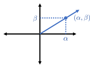
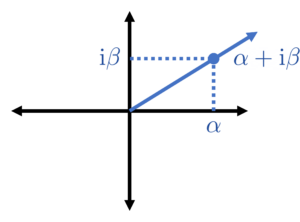
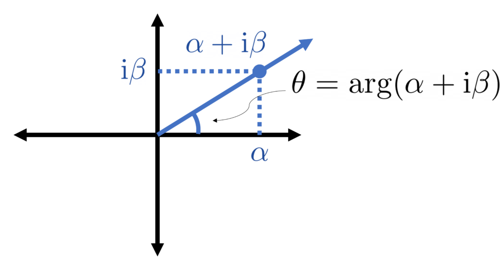
Now comes another standard mathematical trick: represent points in two-dimensional space by complex numbers. In particular, we identify the pair with the complex number  .11Recall that we are assuming that
  is real, so we can pick a scaling in which both and are real numbers. Assume we have done this. Similar to the previous trick, it’s not fully clear why this will pay off, but let’s note it as an insight.
Identify the pair with the complex number .
Now, we combine all the previous observations. The eigenvalue  is best thought of as a pair which, up to scale, can be taken to be and . But then we represent as the complex number

Let’s stop for a moment and appreciate how far we’ve come. The generalized eigenvalue problem is associated with the expression  .If we just went straight from one to the other, this reduction would appear like some crazy stroke of inspiration: why would I ever think to write down ? However, just following our nose lead by a desire to treat and symmetrically and applying a couple standard tricks, this expression appears naturally. The expression will be very useful to us because it is linear in and , and thus for the perturbed problem
  , we have that
  : consequently,
  is a small perturbation of . This observation will be very useful to us.
If is the eigenvector, then the complex number  is .
is .
Definiteness and the Crawford Number
With these insights in hand, we can now return to the point we left earlier about what it means for a generalized eigenvalue problem to be “definite”. We know that if there exists a vector for which , then the problem is singular. If we multiply by , we see that this means that  as well and thus
  . It is thus quite natural to assume the following definiteness condition:
The pair
for all complex nonzero vectors
A definite problem is guaranteed to be not singular, but the reverse is not necessarily true; one can easily find pairs which are not definite and also not singular.12For example, consider  . is not definite since for
  . However, is not singular; the only eigenvalue of the pair is
  and
and  is not identically zero.. (Note does not imply unless and are both positive (or negative) semidefinite.)
The “natural” symmetric condition for to be “definite” is for  for all vectors .
Since the expression  is just scaled by a positive factor by scaling the vector , it is sufficient to check the definiteness condition for only complex unit vectors . This leads naturally to a quantitative characterization of the degree of definiteness of a pair :
The Crawford number13The name Crawford number was coined by G. W. Stewart in 1979 in recognition of Crawford’s pioneering work on the perturbation theory of the definite generalized eigenvalue problem.
of a pair
over all complex unit vectors
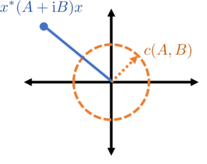
The Crawford number naturally quantifies the degree of definiteness.14In fact, it has been shown that the Crawford number is, in a sense, the distance from a definite matrix pair to a pair which is not simultaneously diagonalizable by congruence. A problem which has a large Crawford number (relative to a perturbation) will remain definite after perturbation, whereas the pair may become indefinite if the size of the perturbation exceeds the Crawford number. Geometrically, the Crawford number has the following interpretation: must lie on or outside the circle of radius centered at  for all (complex) unit vectors .
The “degree of definiteness” can be quantified by the Crawford number  .
.
Now comes another step in our journey which is a bit more challenging. For a matrix  (in our case
  ), the set of complex numbers
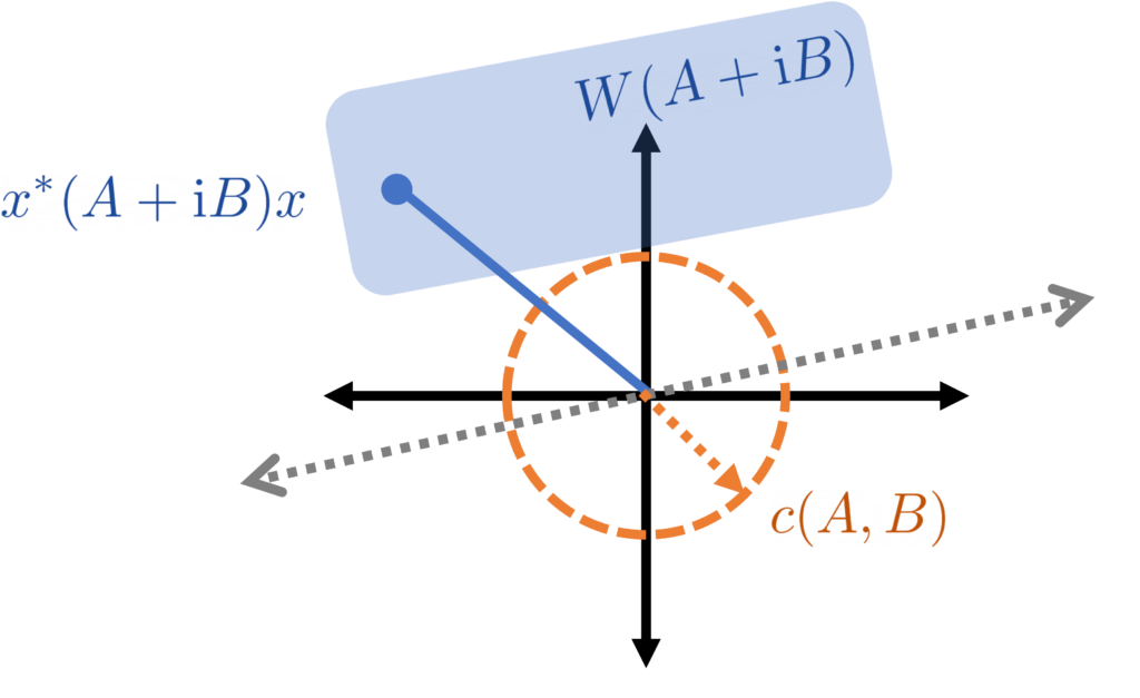
  for all unit vectors has been the subject of considerable study. In fact, this set has a name
The field of values of a matrix
.
In particular, the Crawford number is just the absolute value of the closest complex number in the field of values  to zero.
It is a very cool and highly nontrivial fact (called the Toeplitz–Hausdorff Theorem) that the field of values is always a convex set, with every two points in the field of values containing the line segment connecting them. Thus, as a consequence, the field of values  for a definite matrix pair is always on “one side” of the complex plane (in the sense that there exists a line through zero which lies strictly on one side of15This is a consequence of the hyperplane separation theorem together with the fact that
  .).
.).
The numbers  for unit vectors lie on one half of the complex plane.
 lies outside the circle of radius centered at and thus on one side of the complex plane.
From Eigenvalues to Eigenangles
All of this geometry is lovely, but we need some way of relating it to the eigenvalues. As we observed a while ago, each eigenvalue is best thought of as a ray emanating from the origin, owing to the fact that the pair can be scaled by an arbitrary positive factor. A ray is naturally associated with an angle, so it is natural to characterize an eigenvalue pair by the angle describing its arc.
But the angle of a ray is only defined up additions by full rotations ( radians). As such, to associate each ray a unique angle we need to pin down this indeterminacy in some fixed way. Moreover, this indeterminacy should play nice with the field of values and the field of values
  of the perturbation. But in the last section, we say that each of these field of angles lies (strictly) on one half of the complex plane. Thus, we can find a ray
  which does not intersect either field of values!
One possible choice is to measure the angle from this ray. We shall make a slightly different choice which plays better when we treat as a complex number . Recall that a number  is an argument for if
  for some real number
  . The argument is multi-valued since
  is an argument for
  as long as is (for all integers
  ). However, once we exclude our ray , we can assign each complex number not on this ray a unique argument which depends continuously on . Denote this “branch” of the argument by
  . If represents an eigenvalue , we call
  an eigenangle.
Represent an eigenvalue pair by its associated eigenangle  .
.
How are these eigenangles related to the eigenvalues? It’s now a trigonometry problem:

The eigenvalues are the cotangents of the eigenangles!
The eigenvalue is the cotangent of the eigenangle .
Variational Characterization
Now comes another difficulty spike in our line of reasoning, perhaps the largest in our whole deduction. To properly motivate things, let us first review some facts about the standard Hermitian/symmetric eigenvalue problem. The big idea is that eigenvalues can be thought of as the solution to a certain optimization problem. The largest eigenvalue of a Hermitian/symmetric matrix is given by the maximization problem

The largest eigenvalue is the maximum of the quadratic form over unit vectors . What about the other eigenvalues? The answer is not obvious, but the famous Courant–Fischer Theorem shows that the  th largest eigenvalue
  can be written as the following minimax optimization problem

The minimum is taken over all subspaces  of dimension
  whereas the maximum is taken over all unit vectors within the subspace . Symmetrically, one can also formulate the eigenvalues as a max-min optimization problem

These variational/minimax characterizations of the eigenvalues of a Hermitian/symmetric matrix are essential to perturbation theory for Hermitian/symmetric eigenvalue problems, so it is only natural to go looking for a variational characterization of the generalized eigenvalue problem. There is one natural way of doing this that works for positive definite: specifically, one can show that

This characterization, while useful in its own right, is tricky to deal with because it is nonlinear in and . It also treats and non-symmetrically, which should set off our alarm bells that there might be a better way. Indeed, the ingenious idea, due to G. W. Stewart in 1979, is to instead provide a variational characterization of the eigenangles! Specifically, Stewart was able to show16Stewart’s original definition of the eigenangles differs from ours; we adopt the definition of Mathias and Li. The result amounts to the same thing.
(1) 
for the eigenangles  .17Note that since the cotangent is decreasing on
 ![[0,\pi]](https://www.ethanepperly.com/wp-content/ql-cache/quicklatex.com-37f5d6c600452a51b9fbfc23122f4a36_l3.png "Rendered by QuickLaTeX.com") , this means that the eigenvalues
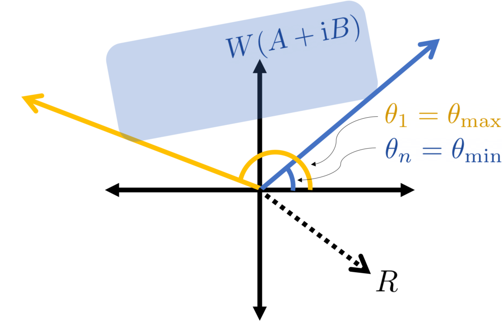
, this means that the eigenvalues  are now in increasing order, in contrast to our convention from earlier in this section. This shows, in particular, that the field of values is subtended by the smallest and largest eigenangles.
The eigenangles satisfy a minimax variational characterization.
How Big is the Perturbation?
We’re tantalizingly close to our objective. The final piece in our jigsaw puzzle before we’re able to start proving perturbation theorems is to quantify the size of the perturbing matrices and . Based on what we’ve done so far, we see that the eigenvalues are natural associated with the complex number , so it is natural to characterize the size of the perturbing pair  by the distance between and
  . But the difference between these two quantities is just

We’re naturally led to the question: how big can  be? If the vector has a large norm, then quite large, so let’s fix to be a unit vector. With this assumption in place, the maximum size of is simple the distance of the farthest point in the field of values
  from zero. This quantity has a name:
The numerical radius of a matrix
(in our case
) is
.18This maximum is taken over all complex unit vectors
The size of the perturbation is the numerical radius  .
.

It is easy to upper-bound the numerical radius  by more familiar quantities. For instance, once can straightforwardly show the bound
  , where
  is the spectral norm. We prefer to state results using the numerical radius because of its elegance: it is, in some sense, the “correct” measure of the size of the pair in the context of this theory.
Stewart’s Perturbation Theory
Now, after many words of prelude, we finally get to our first perturbation theorem. With the work we’ve done in place, the result is practically effortless.
Let  denote the eigenangles of the perturbed pair
  and consider the th eigenangle. Let
  be the subspace of dimension achieving the minimum in the first equation of the variational principle (1) for the original unperturbed pair . Then we have
(2) 
This is something of a standard trick when dealing with variational problems in matrix analysis: take the solution (in this case the minimizing subspace) for the original problem and plug it in for the perturbed problem. The solution may no longer be optimal, but it at least gives an upper (or lower) bound. The complex number must lie at least a distance from zero and  . We’re truly toast if the perturbation is large enough to perturb
  to be equal to zero, so we should assume that
  .
.
For our perturbation theory to work, we must assume .
 lies on or outside the circle centered at zero with radius .
  might lie anywhere in a circle centered at with radius , so one must have to ensure the perturbed problem is nonsingular (equivalently
  for every ).
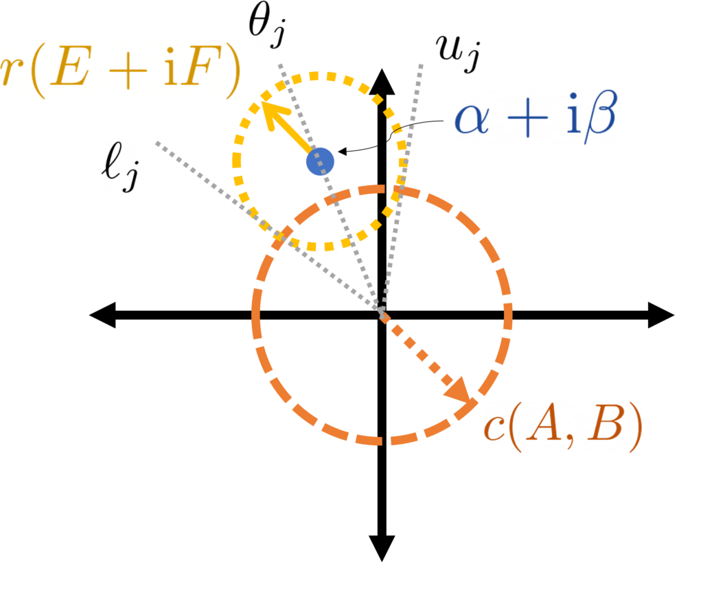
Making the assumption that , bounding the right-hand side of (2) requires finding the most-counterclockwise angle necessary to subtend a circle of radius centered at , which must lie a distance from the origin. The worst-case scenario is when is exactly a distance from the origin, as is shown in the following diagram.
 lies on the circle centered at zero with radius , which is subtended above by angle
  .
.Solving the geometry problem for the counterclockwise-most subtending angle in this worst-case sitation, we conclude the eigenangle bound  . An entirely analogous argument using the max-min variational principle (1) proves an identical lower bound, thus showing
(3) 
In the language of eigenvalues, we have19I’m being a little sloppy here. For a result like this to truly hold, I believe all of the perturbed and unperturbed eigenangles should all be contained in one half of the complex plane.

Interpreting Stewart’s Theory
After much work, we have finally proven our first generalized eigenvalue perturbation theorem. After taking a moment to celebrate, let’s ask ourselves: what does this result tell us?
Let’s start with the good. This result shows us that if the perturbation, measured by the numerical radius  , is much smaller than the definiteness of the original problem, measured by the Crawford number , then the eigenangles change by a small amount. What does this mean in terms of the eigenvalues? For small eigenvalues (say, less than one in magnitude), small changes in the eigenangles also lead to small changes of the eigenvalues. However, for large eigenangles, small changes in the eigenangle are magnified into potentially large changes in the eigenvalues. One can view this result in a positive or negative framing. On the one hand, large eigenvalues could be subject to dramatic changes by small perturbations; on the other hand, the small eigenvalues aren’t “taken down with the ship” and are much more well-behaved.
Stewart’s theory is beautiful. The variational characterization of the eigenangles (1) is a master stroke and exactly the extension one would want from the standard Hermitian/symmetric theory. From the variational characterization, the perturbation theorem follows almost effortlessly from a little trigonometry. However, Stewart’s theory has one important deficit: the Crawford number. All that Stewart’s theory tells is that all of the eigenangles change by at most roughly “perturbation size over Crawford number”. If the Crawford number is quite small since the problem is nearly indefinite, this becomes a tough pill to swallow.
The Crawford number is in some ways essential: if the perturbation size exceeds the Crawford number, the problem can become indefinite or even singular. Thus, we have no hope of fully removing the Crawford number from our analysis. But might it be the case that some eigenangles change by much less than “pertrubation size over Crawford number”? Could we possibly improve to a result of the form “the eigenangles change by roughly perturbation size over something (potentially) much less than the Crawford number”? Sun improved Stewart’s analysis in 1982, but the scourge of the Crawford number remained.20Sun’s bound does not explicitly have the Crawford number, instead using the quantity  and another hard-to-concisely describe quantity. In many cases, one has nothing better to do than to bound
  , in which case the Crawford number has appeared again. The theory of Mathias and Li, published in a technical report in 2004, finally produced a bound where the Crawford number is replaced.
The Mathias–Li Insight and Reduction to Diagonal Form
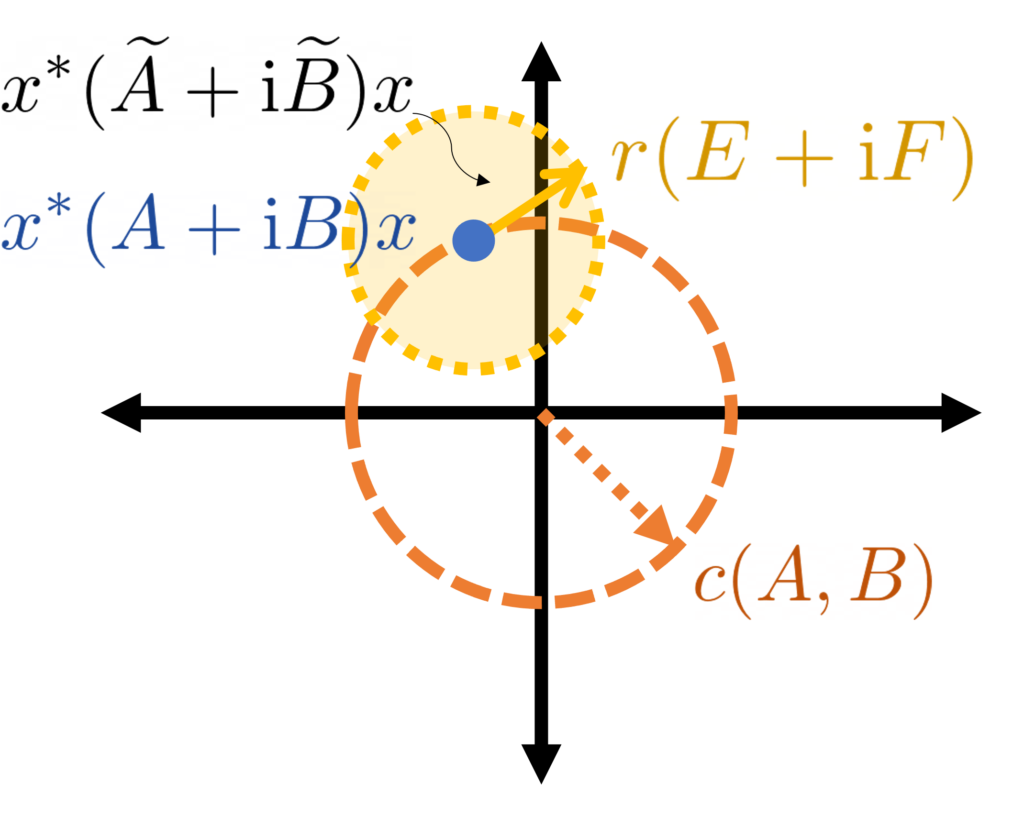
Let’s go back to the Stewart theory and look for a possible improvement. Recall in the Stewart theory that we considered the point on the complex plane. We then argued that, in the worst case, this point would lie a distance from the origin and then drew a circle around it with radius . To improve on Stewart’s bound, we must somehow do something better than using the fact that  . The insight of the Mathias–Li theory is, in some sense, as simple as this: rather than using the fact that
  (as in Stewart’s analysis), use how far actually is from zero, where is chosen to be the unit norm eigenvectors of .21This insight is made more nontrivial by the fact that, in the context of generalized eigenvalue problems, it is often not convenient to choose the eigenvectors to have unit norm. As Mathias and Li note, there are often two more popular normalizations for . If is positive definite, one often normalizes such that
  —the eigenvectors are thus made “-orthonormal”, generalizing the fact that the eigenvectors of a Hermitian/symmetric matrix are orthonormal. Another popular normalization is to scale such that
  . In this way, just taking the eigenvector to have unit norm is already a nontrivial insight.
Before going further, let us quickly make a small reduction which will simplify our lives greatly. Letting  denote a matrix whose columns are the unit-norm eigenvectors of , one can verify that
  and
and  are diagonal matrices with entries
  and
and  respectively. With this in mind, it can make our lives a lot easy to just do a change of variables
  and
and  (which in turn sends
  and
and  ). The change of variables is very common in linear algebra and is called a congruence transformation.
Perform a change of variables by a congruence transformation with the matrix of eigenvectors.
While this change of variables makes our lives a lot easier, we must first worry about how this change of variables might effect the size of the perturbation matrices . It turns out this change of variables is not totally benign, but it is not maximally harmful either. Specifically, the spectral radius can grow by as much as a factor of .22This is because, in virtue of having unit-norm columns, the spectral norm of the matrix is  . Further, note the following variational characterization of the spectral radius
  . Plugging these two facts together yields
  . This factor of isn’t great, but it is much better than if the bound were to degrade by a factor of the condition number
  , which can be arbitrarily large.
This change of variables may increase by at most a factor of .
From now on, we shall tacitly assume that this change of variables has taken place, with and being diagonal and and being such that is at most a factor larger than it was previously. We denote by  and
and  the th diagonal element of and , which are given by
  and
and  where
where  is the th unit-norm eigenvector
Mathias and Li’s Perturbation Theory
We first assume the perturbation is smaller than the Crawford number in the sense , which is required to be assured that the perturbed problem does not lose definiteness. This will be the only place in this analysis where we use the Crawford number.
Draw a circle of radius around  .
.
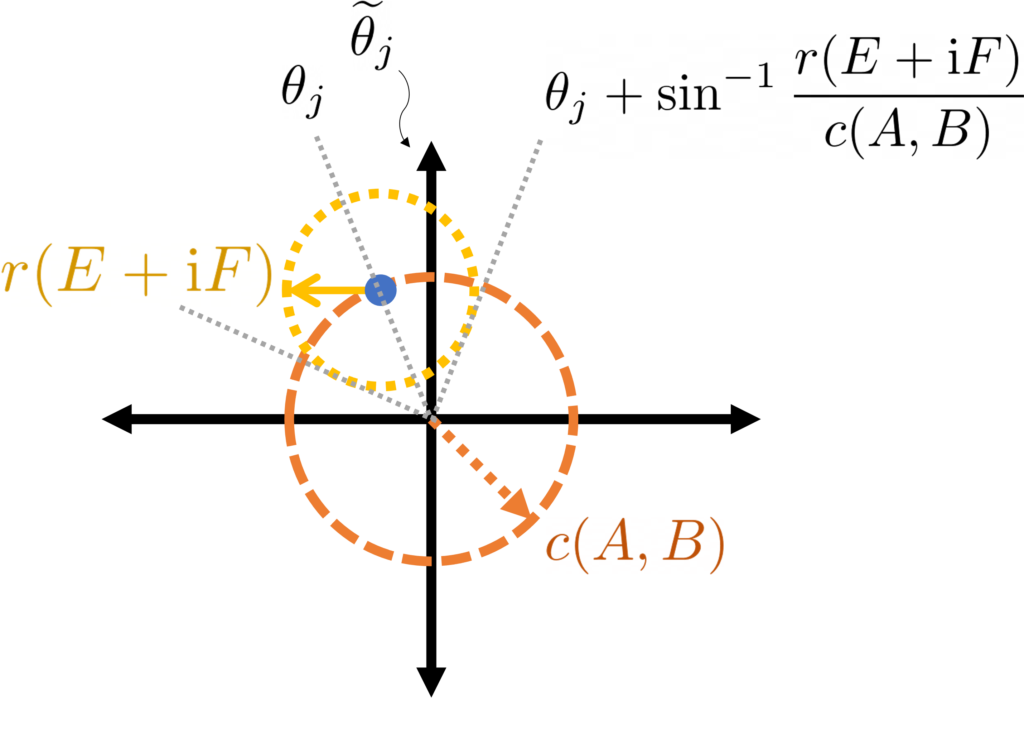
If  is the associated eigenangle, then this circle is subtended by arcs with angles

It would be nice if the perturbed eigenangles  were guaranteed to lie in these arcs (i.e.,
  ). Unfortunately this is not necessarily the case. If one is close to the origin, it will have a large arc which may intersect with other arcs; if this happens, we can’t guarantee that each perturbed eigenangle will remain within its individual arc. We can still say something though.
What follows is somewhat technical, so let’s start with the takeaway conclusion: is larger than any of the lower bounds  . In particular, this means that is larger than the th largest of all the lower bounds. That is, if we rearrange the lower bounds
  in decreasing order
  , we hace
  . An entirely analogous argument will give an upper bound, yielding
(4) 
For those interested in the derivation, read on the in the following optional section:
and are diagonal, the eigenvectors of the pair are just the standard basis vectors, the th of which we will denote  . The trick will be to use the max-min characterization (1) with the subspace spanned by some collection of basis vectors
  . Churning through a couple inequalities in quick fashion,23See pg. 17 of the Mathias and Li report. we obtain

Here,  denotes the convex hull. Since this holds for every set of indices
  , it in particular holds for the set of indices which makes
  the largest. Thus,
  .
.
How to Use Mathias–Li’s Perturbation Theory
The eigenangle perturbation bound (4) can be instantiated in a variety of ways. We briefly sketch two. The first is to bound  by its minimum over all , which then gives a bound on
  (and
(and  )
)

Plugging into (4) and simplifying gives
(5) 
This improves on Stewart’s bound (3) by replacing the Crawford number by  ; as Mathias and Li show is always smaller than or equal to and can be much much smaller.24Recall that Mathias and Li’s bound first requires us to do a change of variables where and both become diagonal, which can increase by a factor of . Thus, for an apples-to-apples comparison with Stewart’s theory where and are non-diagonal, (5) should be interpreted as
  .
.
For the second instantiation (4), we recognize that if an eigenangle is sufficiently well-separated from other eigenangles (relative to the size of the perturbation and ), then we have  and
and  . (The precise instantiation of “sufficiently well-separated” requires some tedious algebra; if you’re interested, see Footnote 7 in Mathias and Li’s paper.25You may also be interested in Corollary 2.2 in this preprint by myself and coauthors.) Under this separation condition, (4) then reduces to
(6) 
This result improves on Stewart’s result (4) by even more, since we have now replaced the Crawford number by  for a sufficiently small perturbation. In fact, a result of this form is nearly as good as one could hope for.26Specifically, the condition number of the eigenangle is
  , so we know for sufficiently small perturbations we have
  and is the smallest number for which such a relation holds. Mathias and Li’s theory allows for a statement of this form to be made rigorous for a finite-size perturbation. Again, the only small deficit is the additional factor of “” from the change of variables to diagonal form.
The Elegant Geometry of Generalized Eigenvalue Perturbation Theory
As I said at the start of this post, what fascinates me about this generalized eigenvalue perturbation is the beautiful and elegant geometry. When I saw it for the first time, it felt like a magic trick: a definite generalized eigenvalue problem with real eigenvalues was transformed by sleight of hand into a geometry problem on the complex plane, with solutions involving just a little high school geometry and trigonometry. Upon studying the theory, I began to appreciate it for a different reason. Upon closer examination, the magic trick was revealed to be a sequence of deductions, each logically following naturally from the last. To the pioneers of this subject—Stewart, Sun, Mathias, Li, and others—this sequence of logical deductions was not preordained, and their discovery of this theory doubtlessly required careful thought and leaps of insight. Now that this theory has been discovered, however, we get the benefit of retrospection, and can retell a narrative of this theory where each step follows naturally from the last. When told this way, one almost imagines being able to develop this theory by oneself, where at each stage we appeal to some notion of mathematical elegance (e.g., by treating and symmetrically) or by applying a standard trick (e.g., identifying a pair with the complex number ). Since this theory took several decades to fall into place, we should not let this storytelling exercise fool us into thinking the prospective act of developing a new theory will be as straightforward and linear as this retelling, pruned of dead ends and halts in progress, might suggest.
That said, I do think the development of the perturbation theory of the generalized eigenvalue problem does have a lesson for those of us who seek to develop mathematical theories: be guided by mathematical elegance. At several points in the development of the perturbation theory, we obtained great gains by treating quantities which play a symmetric role in the problem symmetrically in the theory or by treating a pair of real numbers as a complex number and asking how to interpret that complex number. My hope is that this perturbation theory serves as a good example for how letting oneself be guided by intuition, a small array of standard tricks, and a search for elegance can lead one to conceptualize a problem in the right way which leads (after a considerable amount of effort and a few lucky breaks) to a natural solution.
A truly excellent blog post! The link to Mathias and Li’s technical report from 2004 appears to be broken (in fact, I cannot find it anywhere online). Would you be able to host a copy of the report here, or otherwise send a copy to me directly? Thanks