Today, I want to talk about the generalized Nyström approximation, which I regard as the one of the “big three” approaches to constructing a low-rank approximation to matrix.1The other two approaches are the “projection approximation”/randomized SVD approach and the Nyström approximation. Understanding this approximation, under what conditions it works and the sharpest possible error bounds for it, is a subject of two recent papers of mine:
- Faster Randomized Linear Algebra with Structured Random Matrices, joint with Chris Camaño, Raphael Meyer, and Joel Tropp.
- Sharp analysis of sketched least squares and randomized low-rank approximation, joint with Robert Webber.
On the occasion of the release of the second paper this morning, I felt it was a good time to talk about the generalized Nyström approximation on this blog. In this post, I will try and motivate the generalized Nyström approximation, describing the motivation for the method and when it might be preferable to alternatives.
Existing Characters: Nyström Approximation and the Randomized SVD
To begin our story, let me begin with a reminder of a couple of characters we’ve met in previous installments of this blog, randomized Nyström approximation and the randomized SVD.
Randomized Nyström approximation is a method for producing a low-rank approximation to a positive semidefinite2For this post, a positive semidefinite matrix will always be real symmetric or complex Hermitian. We will focus only on real matrices for this post, though the extension to complex matrices is straightforward. (psd) matrix  . For form this approximation, begin by drawing a random test matrix
  , say, with independent standard normal random entries. (We will have more to say about the choice of below). Using this test matrix, the Nyström approximation is defined as3Here, the inverse
  should be interpreted as a Moore–Penrose pseudoinverse in the event where
  is singular.
![\[\hat{A} = A\Omega (\Omega^\top A\Omega)^{-1} (A\Omega)^\top.\]](https://www.ethanepperly.com/wp-content/ql-cache/quicklatex.com-858ee4e7300bc0e48d12677bd459aeaf_l3.png "Rendered by QuickLaTeX.com")
The randomized SVD is a method for constructing a low-rank approximation to a general, non-symmetric or even non-square matrix  . Again, begin by constructing a random test matrix . To construct a low-rank approximation, compute the product
  and orthonormalize its columns (e.g., by QR decomposition) to obtain
![\[Q \coloneqq \operatorname{orth}(B\Omega).\]](https://www.ethanepperly.com/wp-content/ql-cache/quicklatex.com-77d0237ae3f34369630eff1996a39563_l3.png "Rendered by QuickLaTeX.com")
, yielding the low-rank approximation ![\[\hat{B} = QC \quad \text{for } C = Q^\top B.\]](https://www.ethanepperly.com/wp-content/ql-cache/quicklatex.com-f9906f14f437fa982d3c8a2311d36ee3_l3.png "Rendered by QuickLaTeX.com")
How do these two algorithms compare? There are at least three major differences between the two algorithms. Here are the first two:
- Scope. Nyström approximation applies only to psd matrices, and randomized SVD applies to a general rectangular mtrix.
- Single-pass? The Nyström approximation requires only a single pass over the matrix to form. (Each entry of needs to be read once to form the product
 , after which we have all the information we need from to form
  .) By contrast, the randomized SVD requires two passes, one to compute and a second to compute
  .
.
The third point is more subtle and concerns the accuracy of these algorithms. As we saw in a previous post, the randomized SVD approximation satisfies the error bound
(1) ![\[\expect \norm{B - \hat{B}}_{\rm F}^2 \le \min_{r \le k-2} \left( 1 + \frac{r}{k-(r+1)} \right) \norm{B - \lowrank{B}_r}_{\rm F}^2. \]](https://www.ethanepperly.com/wp-content/ql-cache/quicklatex.com-e3bfd87c8b50495a7a32c42f0af681ac_l3.png "Rendered by QuickLaTeX.com")
 is the matrix Frobenius norm and
  denotes the best rank-
 approximation to . This result, due to Halko, Martinsson, & Tropp (2011), shows that the error of rank-
 randomized SVD is comparable to the error of the best rank- approximation to of any rank
  . See this post for more discussion of this error bound.
Here is analogous bound for the randomized Nyström approximation, taken from Corollary 8.3 in this paper of Tropp and Webber:
(2) ![\[\left(\expect \norm{A - \hat{A}}_{\rm F}^2 \right)^{1/2} \le \min_{r\le k-4} \left(1 + \frac{r+1}{k-(r+3)}\right) \left( \norm{A - \lowrank{A}}_{\rm F} + \frac{1}{\sqrt{k-r}} \norm{A - \lowrank{A}_r}_* \right). \]](https://www.ethanepperly.com/wp-content/ql-cache/quicklatex.com-af14e93166cedc601f5dee4cc4155a7a_l3.png "Rendered by QuickLaTeX.com")
 of the best rank- approximation.
The nuclear norm
![\[\norm{C}_* = \sigma_1(C) + \sigma_2(C) + \cdots\]](https://www.ethanepperly.com/wp-content/ql-cache/quicklatex.com-70e4f079cb458b88416ee8f1c2f9ec2b_l3.png "Rendered by QuickLaTeX.com")
 decrease a slow rate. The matrix with the slowest-possible rate of singular decrease is the identity matrix. For this matrix, its Frobenius is
  , and its nuclear norm is
  —a factor
  larger!
The conclusion of this discussion is that, for matrices with slowly decaying eigenvalues4Recall that the eigenvalues and singular values of a psd matrix coincide., the the randomized Nyström error bound (2) can be much larger than the randomized SVD error bound (1). For such problems, the error of the randomized SVD can be much smaller than the error of randomized Nyström approximation. We add this to our list of comparisons
- Frobenius-norm error bounds? The (Frobenius-norm) error of the randomized SVD
 is bounded in terms of the Frobenius-norm error of the best rank- approximation
  for
for  . For the Nyström approximation, the error
  is bounded by a more complicated expression that also involves the nuclear norm of the best rank- approximation.
Generalized Nyström Approximation: The Best of Both Worlds
It is natural to ask: Is there one algorithm that achieves the positive attributes of both the randomized Nyström and randomized SVD algorithms? Is there a single-pass low-rank approximation algorithm that can be applying to any rectangular matrix and achieves Frobenius-norm error bounds? The answer is yes, and we will derive such an approximation now.
As with the randomized SVD and randomized Nyström approximation, we first compute the product  of with a random matrix . We may then search for the best approximation
  to spanned by the columns of
  . Such an approximation takes the form
  , and we may find the best
  by solving a least-squares problem
(3) ![\[W = \argmin_W \norm{B - YW}_{\rm F}. \]](https://www.ethanepperly.com/wp-content/ql-cache/quicklatex.com-c10c5948a3d56992543344b0490d9a1a_l3.png "Rendered by QuickLaTeX.com")
 , where
  is the Moore–Penrose pseudoinverse. The resulting low-rank approximation is
  . In fact, this approximation coincides with the approximation generated by the randomized SVD algorithm. As with the standard randomized SVD, this approximation takes two passes over to form, one to form and a second to form .
To obtain a one-pass algorithm, we need a faster way of computing an (approximate) solution to the least-squares problem (3). As we have seen before on this blog, sketching provides a natural approach to quickly and approximately solving a least-squares problem. Specifically, we draw another random test matrix  and solve the “sketched” least squares problem
(4) ![\[\hat{W} = \argmin_W \norm{\Phi^\top B - (\Phi^\top Y)W}_{\rm F}. \]](https://www.ethanepperly.com/wp-content/ql-cache/quicklatex.com-e07e026f85c1bc718d95c5c88a47d036_l3.png "Rendered by QuickLaTeX.com")
 of the sketching matrix such be larger than the rank , e.g..
  . The solution to (4) is
 ![\[\hat{W} = (\Phi^\top Y)^\dagger (\Phi^\top B)\]](https://www.ethanepperly.com/wp-content/ql-cache/quicklatex.com-bdf37e0344474a81247242dc1fbc106f_l3.png "Rendered by QuickLaTeX.com")
![\[\hat{B} = Y(\Phi^\top Y)^\dagger (\Phi^\top B) = (B\Omega) (\Phi^\top B\Omega)^\dagger (\Phi^\top B).\]](https://www.ethanepperly.com/wp-content/ql-cache/quicklatex.com-e2fdc92bd90711c249030489953513de_l3.png "Rendered by QuickLaTeX.com")
. (Namely, one should acquire—in the same pass—the products and  .) The generalized Nyström approximation also satisfies our other desired properties, applying to general, rectangular matrix and, as we will see, achieving Frobenius-norm approximation error.
History
In the modern randomized linear algebra literature, the generalized Nyström approximation appears to have been concurrently discovered by Woolfe, Liberty, Rokhlin, & Tygert (2008) and Clarkson & Woodruff (2009). An algebraically equivalent but more numerically stable version of the generalized Nyström approximation was developed by Tropp, Yurtsever, Udell, & Cevher (2017). Nakatsukasa (2020) re-examined the low-rank approximation format, developed a different class of numerical stable implementations, and suggested the name generalized Nyström approximation. Alex Townsend and Per-Gunnar Martinsson trace the origins of this low-rank approximation format far earlier back to the works of Wedderburn (1934).
Implementation
This post is concerned with the generalized Nyström approximation as a type of low-rank approximation format. To use generalized Nyström approximation in practice, one must use an appropriate algorithm which computes the decomposition in a stable way.
Perhaps the simplest algorithm for computing a generalized Nyström approximation was studied by Nakatsukasa (2020). One begins by computing the matrices
![\[Y = B\Omega, \quad Z = B^\top \Omega, \quad C = \Phi^\top Y.\]](https://www.ethanepperly.com/wp-content/ql-cache/quicklatex.com-d95eee60a18e0b58b304b250ab7f3b0f_l3.png "Rendered by QuickLaTeX.com")
as a factored matrix, one takes a QR decomposition  and defines
  and
and  . The generalized Nyström approximation has been computed in factored form:
  . In cases where the core matrix is rank-deficient up to machine precision, the numerical stability of this procedure can sometimes be aided by using a truncated SVD or column-pivoted QR decomposition of ; see Nakatsukasa’s paper for details. An alternate implementation which outputs as a compact SVD was developed by Tropp, Yurtsever, Udell, and Cevher (2017).
Relationship to Other Formats
As the name suggests, the generalized Nyström approximation format generalizes the Nyström approximation beyond psd matrices. Indeed, the standard Nyström approximation
![\[\hat{A} = (A\Omega) (\Omega^\top A \Omega)^\dagger (\Omega^\top A)\]](https://www.ethanepperly.com/wp-content/ql-cache/quicklatex.com-fb7ae8960f8c0173063c23f7290a1b63_l3.png "Rendered by QuickLaTeX.com")
with a test matrix  .
.
Perhaps less obviously, the generalized Nyström approximation also generalizes the randomized SVD approximation. Indeed, the randomized SVD approximation  is the generalized Nyström approximation with trivial right test matrix
  .
.
Generalized Nyström Approximation = Sketch-and-Solve + Randomized SVD
What is the generalized Nyström approximation? There are several interpretations. For instance, if  and
and  is invertible, the generalized Nyström approximation is the unique approximation satisfying the interpolatory condition
![\[\hat{B}\Omega = B\Omega \quad \text{and} \quad \hat{B}^\top\Phi = B^\top\Phi.\]](https://www.ethanepperly.com/wp-content/ql-cache/quicklatex.com-ed39d951ca827f023b0460fce18b1e0a_l3.png "Rendered by QuickLaTeX.com")
Notwithstanding the validity and usefulness of other interpretations, my view is that the most useful interpretation of generalized Nyström approximation is the one we started with:
Generalized Nyström approximation is a sketched version of the randomized SVD approximation.
To see this insight in action, we will use it to analyze the generalized Nyström approximation with Gaussian test matrices. Let  and be populated with independent standard Gaussian random entries, and as we have been, assume
  . Let us analyze the expected (squared) Frobenius-norm error of the generalized Nyström approximation.
We will use the following result for sketching with a Gaussian embedding, due to Bartan & Pilanci (2020) and discussed in this previous blog post.
Theorem 1 (sketch-and-solve): Consider a (matrix) least-squares problem
with dimensions
and
. Let
Then
![\[W = Y^\dagger B= \argmin_W \norm{B - YW}_{\rm F}\]](https://www.ethanepperly.com/wp-content/ql-cache/quicklatex.com-1fbec03b765e920f2546d70acc1e315d_l3.png "Rendered by QuickLaTeX.com")
![\[\hat{W} = (\Phi^\top Y)^\dagger \Phi^\top B = \argmin_W \norm{\Phi^\top B - (\Phi^\top Y)W}_{\rm F}.\]](https://www.ethanepperly.com/wp-content/ql-cache/quicklatex.com-47453e73c76d516332da7709bec4fdf2_l3.png "Rendered by QuickLaTeX.com")
![\[\expect \norm{B - Y\hat{W}}_{\rm F}^2 = \expect \norm{B - Y(\Phi^\top Y)^\dagger\Phi^\top B}_{\rm F}^2 = \left( 1 + \frac{k}{p - (k+1)} \right)\norm{B - YY^\dagger B}_{\rm F}^2.\]](https://www.ethanepperly.com/wp-content/ql-cache/quicklatex.com-1dd58766c5711cb52838468de28f2956_l3.png "Rendered by QuickLaTeX.com")
We can apply this result to the generalized Nyström approximation by setting . Let  denote the expectation over
  alone. Then
![\[\expect_\Phi \norm{B - B\Omega(\Phi^\top B\Omega)^\dagger\Phi^\top B}_{\rm F}^2 = \left( 1 + \frac{k}{p - (k + 1)} \right)\norm{B - (B\Omega)(B\Omega)^\dagger B}_{\rm F}^2.\]](https://www.ethanepperly.com/wp-content/ql-cache/quicklatex.com-3ca90719321990c2e97c775f86238ce7_l3.png "Rendered by QuickLaTeX.com")
 is just the randomized SVD approximation. Invoking the randomized SVD bound (1) yields
 ![\begin{align*}\expect \norm{B - B\Omega(\Phi^\top B\Omega)^\dagger\Phi^\top B}_{\rm F}^2 &= \expect_\Omega\left[\expect_\Phi \norm{B - B\Omega(\Phi^\top B\Omega)^\dagger\Phi^\top B}_{\rm F}^2\right] \\&= \left( 1 + \frac{k}{p - (k + 1)} \right)\expect_\Omega \norm{B - (B\Omega)(B\Omega)^\dagger B}_{\rm F}^2 \\&\le \left( 1 + \frac{k}{p - (k + 1)} \right)\left[\min_{r < k-1}\left( 1 + \frac{r}{k - (r + 1)} \right) \norm{B - \lowrank{B}_r}_{\rm F}^2\right].\end{align*}](https://www.ethanepperly.com/wp-content/ql-cache/quicklatex.com-f6a0cfb074737e67fcb3b172f5d5badc_l3.png "Rendered by QuickLaTeX.com")
Theorem 2 (generalized Nyström approximation): With the present setting, it holds that
![\[\expect \norm{B - B\Omega(\Phi^\top B\Omega)^\dagger\Phi^\top B}_{\rm F}^2 \le \left( 1 + \frac{k}{p - (k + 1)} \right)\left[\min_{r < k-1}\left( 1 + \frac{r}{k - (r + 1)} \right) \norm{B - \lowrank{B}_r}_{\rm F}^2\right].\]](https://www.ethanepperly.com/wp-content/ql-cache/quicklatex.com-be78edd2761af9a1cc467056a24c73e9_l3.png "Rendered by QuickLaTeX.com")
This result is Theorem 4.3 in this paper of Tropp, Yurtsever, Udell, & Cevher (2017). A slight refinement of this bound appears in my paper with Robert Webber, and we show that our new bound is sharp on hard examples. Thus, Theorem 2 is nearly the best possible error bound for the generalized Nyström approximation.
Choice of Random Matrix
For most of this post, we have focused on the cases where the random test matrices and are unstructured matrices with Gaussian random entries. But can we use more structured random test matrices? Say, sparse test matrices? Do these lead to faster low-rank approximation algorithms?
For the randomized SVD, the results are disappointing. Computing with a sparse random matrix is fast. But then we compute  and compute
  ; the matrix
  is dense and unstructured, so computing is slower and all benefits of the sparse test matrix have been erased.
The issue with the randomized SVD is that it’s a two-pass algorithm: The first pass, computing , can be done using a sparse random test matrix. But the second pass requires a matrix product with a dense matrix .
The situation is much better for the generalized Nyström approximation, which requires only a single pass and can be implemented only by multiplying against sparse matrices. Indeed, generating and to be sparse matrices, the generalized Nyström approximation can be written
![\[\hat{B} = Y(\Phi^* Y)^\dagger Z \quad \text{for } Y = B\Omega \text{ and } Z = \Phi^\top B.\]](https://www.ethanepperly.com/wp-content/ql-cache/quicklatex.com-959c9e287d25f46bd1011f38affcab7b_l3.png "Rendered by QuickLaTeX.com")
has been isolated into matrix products with the random test matrices, and we obtain speedups by replacing using sparse random test matrices for and .
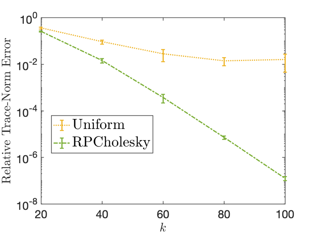
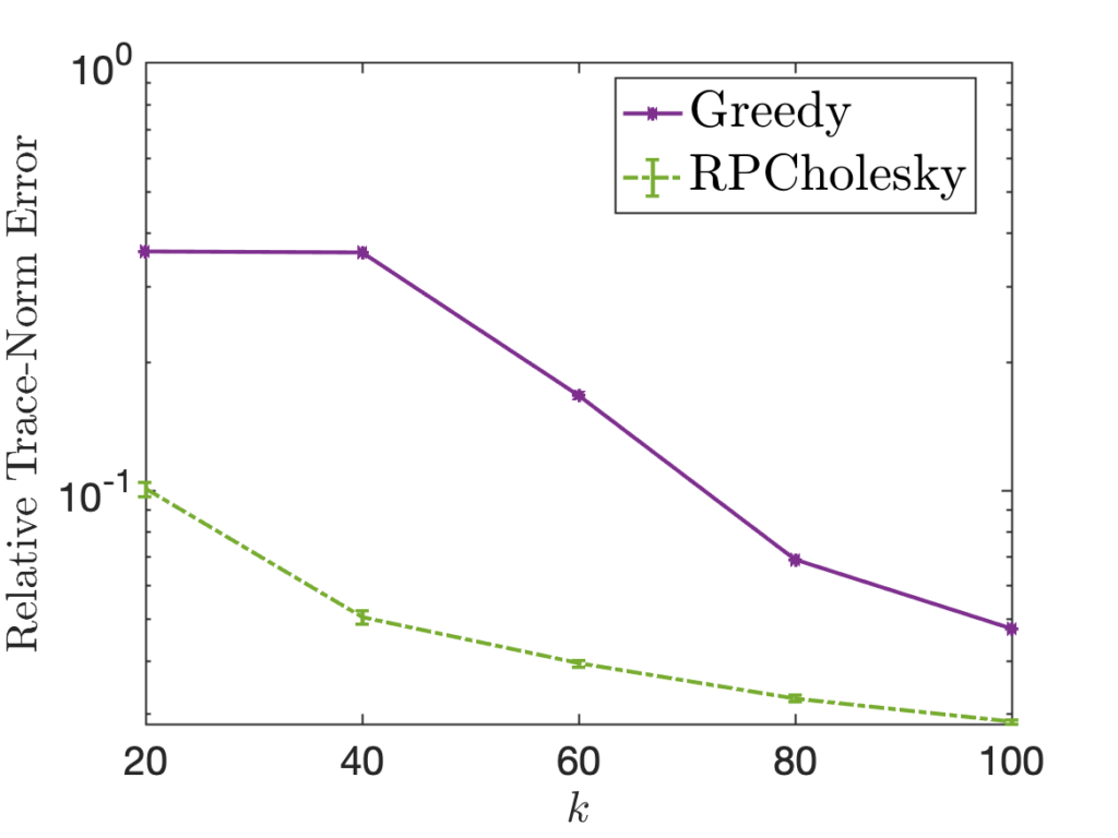
Structured test matrices, like sparse ones, can be very powerful. But basic theoretical questions remain about their properties. We tackle these theoretical questions in my new paper (joint with Chris Camaño, Raphael Meyer, and Joel Tropp), and we provide experiments demonstrating how structured sketching matrices can lead to large speedups in generalized Nyström approximation and other linear algebra tasks. I think it’s a really neat paper, and my wonderful collaborator Chris did some really beautiful experiments for it. I hope you’ll check it out!
 , one of the standard techniques is the standard
  .
. .
. .
. for
for  .
. , where
  denotes the
  . This motivates the general definition:
 is one that is symmetric and possesses nonnegative
  ; we will have much more to say about Gram matrices below.
![\[\hat{A} \coloneqq (A\Omega) (\Omega^\top A \Omega)^{-1}(A\Omega)^\top.\]](https://www.ethanepperly.com/wp-content/ql-cache/quicklatex.com-324f22320951777dd4f468db63441a88_l3.png "Rendered by QuickLaTeX.com")
 be any rectangular matrix and consider the Gram matrix
  to
to  to
to ![\[\hat{A} = \smash{\hat{B}}^\top \hat{B}.\]](https://www.ethanepperly.com/wp-content/ql-cache/quicklatex.com-d117cb87f2d340e70cf67c27d22eda9b_l3.png "Rendered by QuickLaTeX.com")
 of the projection approximation
  is the Nyström approximation
  .
.
 is a projection matrix, it satisfies
  . Thus,
 ![\[\hat{B}^\top \hat{B} = B^\top \Pi_{B\Omega}^2B = B^\top \Pi_{B\Omega}B.\]](https://www.ethanepperly.com/wp-content/ql-cache/quicklatex.com-48bef2e2a5d8c3d62885c4d9b401657a_l3.png "Rendered by QuickLaTeX.com")
 . Using this formula, we obtain
 ![\[\hat{B}^\top \hat{B} = B^\top B\Omega (\Omega^\top B^\top B \Omega)^{-1} \Omega^\top B^\top B.\]](https://www.ethanepperly.com/wp-content/ql-cache/quicklatex.com-d23468b24025dc8e100c51d6529cd298_l3.png "Rendered by QuickLaTeX.com")
 , confirming the Gram correspondence.
 generated by every matrix
  with orthonormal columns. This motivates the following definition:
 . Indeed, a Gram square root
  need not even be defined.
 . The matrix square root
  . Moreover, it is the unique matrix with these properties.
 .
. and use following formula:
![\[\hat{A} = Y (\Omega^\top Y)^{-1} Y^\top.\]](https://www.ethanepperly.com/wp-content/ql-cache/quicklatex.com-26a3012188a11c08b56517e952560fa8_l3.png "Rendered by QuickLaTeX.com")
 . The randomized SVD approximation
  . For
. For  , perform the following steps:
 . These indices are referred to as
 ![\[\hat{A} \gets \hat{A} + \frac{A(:,s_i)A(s_i,:)}{A(s_i,s_i)}.\]](https://www.ethanepperly.com/wp-content/ql-cache/quicklatex.com-ec07289a72875184db6bb7476af3149e_l3.png "Rendered by QuickLaTeX.com")
![\[A \gets A - \frac{A(:,s_i)A(s_i,:)}{A(s_i,s_i)}.\]](https://www.ethanepperly.com/wp-content/ql-cache/quicklatex.com-0f9632b22fb854d1c90533858afc4321_l3.png "Rendered by QuickLaTeX.com")
![\[\hat{A} = A(:,S) A(S,S)^{-1} A(S,:),\]](https://www.ethanepperly.com/wp-content/ql-cache/quicklatex.com-a2ee3b57f3e6b12a8a43ba694d856650_l3.png "Rendered by QuickLaTeX.com")
 . This type of low-rank approximation is known as a
  equal to a subset of columns of the identity matrix
  . For an explanation of why this procedure is called a “pivoted partial Cholesky decomposition” and the relation to the usual notion of Cholesky decomposition, see
  . For
. For  .
. .
. , which is an example of the general projection approximation with
  , where
  is an upper trapezoidal matrix, up to a permutation of the rows. This factorized form is easy to compute roughly following steps 1–3 above, which explains why we call that procedure a “
 for a weight matrix
  . This type of factorization is known as an
  , and compute a column Nyström approximation
  .
.![\[\prob\{s_i = j\} = \frac{\norm{B(:,j)}^2}{\norm{B}_{\rm F}^2} \quad \text{for } j=1,2,\ldots,k.\]](https://www.ethanepperly.com/wp-content/ql-cache/quicklatex.com-9dd2bd2b1a2336439460e2d9edc93ac1_l3.png "Rendered by QuickLaTeX.com")
 .
. operations, so the full procedure requires
  operations. This makes the cost of the algorithm similar to other methods for rectangular low-rank approximation such as the randomized SVD, but it has the advantage that it computes a column projection approximation.
 of
of ![\[\norm{B(:,j)}^2 = B(:,j)^\top B(:,j) = (B^\top B)(j,j) = A(j,j).\]](https://www.ethanepperly.com/wp-content/ql-cache/quicklatex.com-61799b78022402815125a4a4838a0790_l3.png "Rendered by QuickLaTeX.com")
 . Therefore, we can write the probability distribution for the random pivot
 ![\[\prob\{s_i = j\} = \frac{A(j,j)}{\tr A} \quad \text{for } j=1,2,\ldots,N.\]](https://www.ethanepperly.com/wp-content/ql-cache/quicklatex.com-7e86c11c687ad0dbec8ce551cbf91e5b_l3.png "Rendered by QuickLaTeX.com")
 is
is ![\[\hat{A} &\gets \left(\hat{B} + \frac{B(:,s_i) (B(:,s_i)^\top B)}{\norm{B(:,s_i)}^2}\right)^\top \left(\hat{B} + \frac{B(:,s_i) (B(:,s_i)^\top B)}{\norm{B(:,s_i)}^2}\right).\]](https://www.ethanepperly.com/wp-content/ql-cache/quicklatex.com-d691d56d7580112fdd2d2db8eb4cd4aa_l3.png "Rendered by QuickLaTeX.com")
 , this simplifies to
  The matrix
  , leading the second and third term to vanish. Finally, using the relation
![\[\hat{A} \gets \hat{A} +\frac{A(:,s_i)A(s_i,:)}{A(s_i,s_i)}.\]](https://www.ethanepperly.com/wp-content/ql-cache/quicklatex.com-20c81e35e173568377cad3b27f62062e_l3.png "Rendered by QuickLaTeX.com")
![\[A \gets A -\frac{A(:,s_i)A(s_i,:)}{A(s_i,s_i)}.\]](https://www.ethanepperly.com/wp-content/ql-cache/quicklatex.com-3c79822c70c086025440e38f0561169f_l3.png "Rendered by QuickLaTeX.com")
![\[\prob\{s_i = j\} = \frac{A(j,j)}{\tr(A)} \quad \text{for } j=1,2,\ldots,k.\]](https://www.ethanepperly.com/wp-content/ql-cache/quicklatex.com-750f3165cab9fdf250259d6e294fabfc_l3.png "Rendered by QuickLaTeX.com")
 and through the diagonal entries
  . Therefore, we can derive an optimized version of the randomly pivoted Cholesky algorithm that only reads
  entries of the matrix
  operations! See
  operations, and we used it to derive the randomly pivoted Cholesky algorithm that runs in
  operations. Let’s make this concrete with some specific numbers. Setting
  and
and  , randomly pivoted QR requires roughly
  (100 trillion) operations and randomly pivoted Cholesky requires roughly
  (10 billion) operations, a factor of 10,000 smaller operation count!
 as output.
![\[\norm{B - \hat{B}}_{\rm F}^2 = \tr(A - \hat{A}).\]](https://www.ethanepperly.com/wp-content/ql-cache/quicklatex.com-2d3c7ab4822ad680c4e24c9044d05a1c_l3.png "Rendered by QuickLaTeX.com")

 is nonnegative and satisfies
  if and only if
  ; these statements justify why
  is an appropriate expression for measuring the error of the approximation
  .
.![\[\expect \norm{B - \hat{B}}_{\rm F}^2 \le \min_{r\le k-2} \left(1 + \frac{r}{k-(r+1)} \right) \norm{B - \lowrank{B}_r}_{\rm F}^2,\]](https://www.ethanepperly.com/wp-content/ql-cache/quicklatex.com-6a686d8b6380eeb6efbbeb877462b6fc_l3.png "Rendered by QuickLaTeX.com")
 . Using the transference principle, we immediately obtain a corresponding bound for rank-
 . This identity, too, follows by the transference principle, since
  are, themselves, projection approximations and Nyström approximations corresponding to choosing
 ![\[\expect \tr(A - \hat{A}) \le \min_{r\le k-2} \left(1 + \frac{r}{k-(r+1)} \right) \tr(A - \lowrank{A}_r).\]](https://www.ethanepperly.com/wp-content/ql-cache/quicklatex.com-147e2f2f5939fab29eb3e90e42bf3bb9_l3.png "Rendered by QuickLaTeX.com")
 is
is ![\[\norm{UCV}_{\rm UI} = \norm{C}_{\rm UI}\]](https://www.ethanepperly.com/wp-content/ql-cache/quicklatex.com-508a8e72c2095a615973294b1ae77137_l3.png "Rendered by QuickLaTeX.com")
 .
. , the Frobenius norm
  , and the spectral norm
  . (It is not coincidental that all these unitarily invariant norms can be expressed only in terms of the singular values
  of the matrix
 ![\[\norm{C}_{\rm Q}^2 = \norm{C^\top C}_{\rm UI} = \norm{CC^\top}_{\rm UI}.\]](https://www.ethanepperly.com/wp-content/ql-cache/quicklatex.com-defbf79c07f9c16df2fd2362255e9cb3_l3.png "Rendered by QuickLaTeX.com")
 is the Frobenius norm
  .
. .
.![\[\norm{B - \hat{B}}_{\rm Q}^2 = \norm{A - \hat{A}}\]](https://www.ethanepperly.com/wp-content/ql-cache/quicklatex.com-b4db0757c230531d100a996ea48eb1c5_l3.png "Rendered by QuickLaTeX.com")
 .
.
![\[\norm{B - \hat{B}}_{\rm F}^2 = \norm{A - \hat{A}}_* = \tr(A - \hat{A}).\]](https://www.ethanepperly.com/wp-content/ql-cache/quicklatex.com-3e89aa937f513384f415603332de4c86_l3.png "Rendered by QuickLaTeX.com")
![\[\norm{B - \hat{B}}^2 = \norm{A - \hat{A}}.\]](https://www.ethanepperly.com/wp-content/ql-cache/quicklatex.com-f93fc86775f946e645a8df65f928aaef_l3.png "Rendered by QuickLaTeX.com")
 . Thus,
 ![\[\norm{B - \hat{B}}_{\rm Q}^2 = \norm{(I-\Pi_{B\Omega})B}_{\rm Q}^2 = \norm{B^\top (I-\Pi_{B\Omega})^2B}_{\rm UI}.\]](https://www.ethanepperly.com/wp-content/ql-cache/quicklatex.com-41bc10e5110325aa263b549e0265f3f4_l3.png "Rendered by QuickLaTeX.com")
 are equal to their own square, so
![\[\norm{B - \hat{B}}_{\rm Q}^2 = \norm{A - \hat{A}}_{\rm UI},\]](https://www.ethanepperly.com/wp-content/ql-cache/quicklatex.com-1f34c55899f793cae1721f2e19e002bc_l3.png "Rendered by QuickLaTeX.com")
 the rank-
 measured in some
  ? What about expected squared error
  ? How do these answers change with different norms?
 get except for some small failure probability
  ?
? compared to the best rank-
![\[\mathbb{E} \left\|B-X\right\|_{\rm F}^2 \le \left( 1 + \frac{k}{k-(r+1)}\right) \left\|B - \lowrank{B}_r \right\|_{\rm F}^2 \quad \text{for every $r \le k-2$}.\]](https://www.ethanepperly.com/wp-content/ql-cache/quicklatex.com-6759ab11982f765f19dc615fb8e1fbdc_l3.png "Rendered by QuickLaTeX.com")
 is the
  random matrix.
 , where
  denotes the
 ![\[B\approx X \coloneqq QC.\]](https://www.ethanepperly.com/wp-content/ql-cache/quicklatex.com-dbf0ef5be3e2a7fc39d609f4621d2dbd_l3.png "Rendered by QuickLaTeX.com")
 into a
  , as we did as steps 4 and 5 in the previous post.
![\[X = QC = QQ^*B = \Pi_{B\Omega} B.\]](https://www.ethanepperly.com/wp-content/ql-cache/quicklatex.com-0d1ae78fbe7d6d4d91b567795bd91f57_l3.png "Rendered by QuickLaTeX.com")
 the projection formula for the randomized SVD.
![\[U^*U = UU^* = I.\]](https://www.ethanepperly.com/wp-content/ql-cache/quicklatex.com-33fedf7ef9e12832ea6188011e3874bd_l3.png "Rendered by QuickLaTeX.com")
 on matrices is
 ![\[\left\|UBV\right\|_{\rm UI} = \left\|B\right\|_{\rm UI} \quad \text{for all unitary matrices $U$, $V$ and any matrix $B$}.\]](https://www.ethanepperly.com/wp-content/ql-cache/quicklatex.com-5fd16f43277f7e25ee2f910665984e09_l3.png "Rendered by QuickLaTeX.com")
 is said to be quadratic if there exists another unitarily invariant norm
 ![\[\left\|B\right\|_{\rm Q}^2 = \left\|B^*B\right\|_{\rm UI} = \left\|BB^*\right\|_{\rm UI} \quad \text{for every matrix $B$.} \]](https://www.ethanepperly.com/wp-content/ql-cache/quicklatex.com-aac3c6aec691fb438adf6690682d855d_l3.png "Rendered by QuickLaTeX.com")
![\[\left\|B\right\|_{S_p}^p \coloneqq \sum_i \sigma_i(B)^p.\]](https://www.ethanepperly.com/wp-content/ql-cache/quicklatex.com-d032386a33d5df74c8a44235dafac359_l3.png "Rendered by QuickLaTeX.com")
 denote the decreasingly order
  -norm
-norm  is the
  -norm, defined to be
![\[\norm{B} = \left\|B\right\|_{S_\infty} \coloneqq \max_i \sigma_i(B) = \sigma_1(B).\]](https://www.ethanepperly.com/wp-content/ql-cache/quicklatex.com-584051e6c083d9b865ffe52d79186a00_l3.png "Rendered by QuickLaTeX.com")
 . However, the Schatten
  since
since![\[\left\|B\right\|_{S_p}^2 = \left\|B^*B\right\|_{S_{p/2}}.\]](https://www.ethanepperly.com/wp-content/ql-cache/quicklatex.com-27e888ecff0b0c38df6e73a803f8aa1d_l3.png "Rendered by QuickLaTeX.com")
![\[\left\|B - X\right\|_{\rm Q}^2 \le \left\|B - \lowrank{B}_r\right\|_{\rm Q}^2 + \left\|\lowrank{B}_r - \Pi_{B\Omega} \lowrank{B}_r\right\|_{\rm Q}^2. \]](https://www.ethanepperly.com/wp-content/ql-cache/quicklatex.com-c1738a10a5c46d5455b8e2d5992ce98d_l3.png "Rendered by QuickLaTeX.com")
![\[\left\|B - \lowrank{B\right\|_r}_{\rm Q} \le \left\|B - C\right\|_{\rm Q} \quad \text{for any rank-$r$ matrix $C$}.\]](https://www.ethanepperly.com/wp-content/ql-cache/quicklatex.com-46106e1ebeaa349721ea4e81d171f70b_l3.png "Rendered by QuickLaTeX.com")
![\[\left\|B - X\right\|_{\rm Q}^2 - \left\|B - \lowrank{B}_r\right\|_{\rm Q}^2 \le \left\|\lowrank{B}_r - \Pi_{B\Omega} \lowrank{B}_r\right\|_{\rm Q}^2.\]](https://www.ethanepperly.com/wp-content/ql-cache/quicklatex.com-e44e6de74ec072bf3d6c944ea6de77db_l3.png "Rendered by QuickLaTeX.com")

 is an orthoprojector and thus has unit spectral norm
  together with the fact that
![\[\left\|BCD\right\|_{\rm UI} \le \norm{B} \cdot \left\|C\right\|_{\rm UI}\cdot \norm{D} \quad \text{for all matrices $B,C,D$.}\]](https://www.ethanepperly.com/wp-content/ql-cache/quicklatex.com-e329f332e4305af288668bfdf1ab4bf5_l3.png "Rendered by QuickLaTeX.com")
![\[(B - \lowrank{B}_r)(B - \lowrank{B}_r)^* = BB^* - \lowrank{B}_r\lowrank{B}_r^*.\]](https://www.ethanepperly.com/wp-content/ql-cache/quicklatex.com-9db3f7e6eb57261b556783a0a7d62fd0_l3.png "Rendered by QuickLaTeX.com")
![\[B = \onebytwo{U_1}{U_2} \twobytwo{\Sigma_1}{0}{0}{\Sigma_2}\onebytwo{V_1}{V_2}^*\]](https://www.ethanepperly.com/wp-content/ql-cache/quicklatex.com-54a749c18b5a76a0f468adee8b5fa58f_l3.png "Rendered by QuickLaTeX.com")
 and
and  both have orthonormal columns,
 and
and  are square diagonal matrices with nonnegative entries,
 and
and  have
have  matrix.
 . Define
![\[\twobyone{\Omega_1}{\Omega_2} \coloneqq \twobyone{V_1^*}{V_2^*} \Omega.\]](https://www.ethanepperly.com/wp-content/ql-cache/quicklatex.com-f620ec79bd8a3f6022efb5ca07b0d824_l3.png "Rendered by QuickLaTeX.com")
 is full-rank (i.e.,
  ).
).
 so
so![\[\norm{(I-\Pi_{B\Omega})U_1\Sigma_1}_{\rm Q}^2 \le \norm{(I-\Pi_{B\Omega\Omega_1^\dagger})U_1\Sigma_1}_{\rm Q}^2 = \norm{\Sigma_1U_1^*(I-\Pi_{B\Omega\Omega_1^\dagger})U_1\Sigma_1}_{\rm UI}. \]](https://www.ethanepperly.com/wp-content/ql-cache/quicklatex.com-2fdd85edd3e561ae5496031960d8901a_l3.png "Rendered by QuickLaTeX.com")
![\[\Sigma_1U_1^*(I-\Pi_{B\Omega\Omega_1^\dagger})U_1\Sigma_1.\]](https://www.ethanepperly.com/wp-content/ql-cache/quicklatex.com-f21f88902abb8532d54b098fa358ddc0_l3.png "Rendered by QuickLaTeX.com")
![\[B\Omega\Omega_1^\dagger = B\onebytwo{V_1}{V_2}\twobyone{\Omega_1}{\Omega_2}\Omega_1^\dagger = \onebytwo{U_1}{U_2} \twobytwo{\Sigma_1}{0}{0}{\Sigma_2} \twobyone{I}{\Omega_2\Omega_1^\dagger} = U_1\Sigma_1 + U_2\Sigma_2\Omega_2\Omega_1^\dagger.\]](https://www.ethanepperly.com/wp-content/ql-cache/quicklatex.com-e1dbcff75c12101b6274492896899b52_l3.png "Rendered by QuickLaTeX.com")
 takes the form
![\begin{align*}\Pi_{B\Omega\Omega_1^\dagger} &= (B\Omega\Omega_1^\dagger) \left[(B\Omega\Omega_1^\dagger)^*(B\Omega\Omega_1^\dagger)\right]^\dagger (B\Omega\Omega_1^\dagger)^* \\&= (U_1\Sigma_1 + U_2\Sigma_2\Omega_2\Omega_1^\dagger) \left[\Sigma_1^2 + (\Sigma_2\Omega_2\Omega_1^\dagger)^*(\Sigma_2\Omega_2\Omega_1^\dagger)\right]^\dagger (U_1\Sigma_1 + U_2\Sigma_2\Omega_2\Omega_1^\dagger)^*.\end{align*}](https://www.ethanepperly.com/wp-content/ql-cache/quicklatex.com-d9e0cd585357787c460f6471f52ecb0a_l3.png "Rendered by QuickLaTeX.com")
![\[\Sigma_1U_1^*(I-\Pi_{B\Omega\Omega_1^\dagger})U_1\Sigma_1 = \Sigma_1^2 - \Sigma_1^2 \left[\Sigma_1^2 + (\Sigma_2\Omega_2\Omega_1^\dagger)^*(\Sigma_2\Omega_2\Omega_1^\dagger)\right]^\dagger\Sigma_1^2. \]](https://www.ethanepperly.com/wp-content/ql-cache/quicklatex.com-b7dfa3f3cbcda5380b6b7ec0132fca2a_l3.png "Rendered by QuickLaTeX.com")
 is defined as
![\[A : H \coloneqq A - A(A+H)^\dagger A. \]](https://www.ethanepperly.com/wp-content/ql-cache/quicklatex.com-0ca6dd2810aa560e0d59d808c9b40bc8_l3.png "Rendered by QuickLaTeX.com")
![\[\Sigma_1U_1^*(I-\Pi_{B\Omega\Omega_1^\dagger})U_1\Sigma_1 = \Sigma_1^2 : [(\Sigma_2\Omega_2\Omega_1^\dagger)^*(\Sigma_2\Omega_2\Omega_1^\dagger)].\]](https://www.ethanepperly.com/wp-content/ql-cache/quicklatex.com-dc620e38c4fb8a7855e330183c8313c9_l3.png "Rendered by QuickLaTeX.com")
![\[\left\|B - X\right\|_{\rm Q}^2\le \left\| \Sigma_2 \right\|_{\rm Q}^2 + \left\|\Sigma_1^2 : [(\Sigma_2\Omega_2\Omega_1^\dagger)^*(\Sigma_2\Omega_2\Omega_1^\dagger)]\right\|_{\rm UI}. \]](https://www.ethanepperly.com/wp-content/ql-cache/quicklatex.com-ff8a161c38344c97e0d615d216d4555d_l3.png "Rendered by QuickLaTeX.com")
 and we connect the ends using a wire of
  . The
. The  is given by
 ![\[v = a \cdot \mathrm{curr}_a.\]](https://www.ethanepperly.com/wp-content/ql-cache/quicklatex.com-50ff6a1f099e535f6dfd8525f45b4741_l3.png "Rendered by QuickLaTeX.com")
 , the current
  is then
![\[v = h \cdot \mathrm{curr}_h.\]](https://www.ethanepperly.com/wp-content/ql-cache/quicklatex.com-baea64abba5be2425a04d7d2316f7153_l3.png "Rendered by QuickLaTeX.com")
![\[\mathrm{curr}_{\rm total} = \mathrm{curr}_a + \mathrm{curr}_h = \frac{v}{a} + \frac{v}{h} = v \left(a^{-1}+h^{-1}\right).\]](https://www.ethanepperly.com/wp-content/ql-cache/quicklatex.com-2ce6cd66280641977f8eea4d3d9f6cab_l3.png "Rendered by QuickLaTeX.com")
![\[a:h \coloneqq \frac{v}{\mathrm{curr}_{\rm total}} = \left( a^{-1}+h^{-1}\right)^{-1}. \]](https://www.ethanepperly.com/wp-content/ql-cache/quicklatex.com-46eba66bdf328c974e763d8c43422e75_l3.png "Rendered by QuickLaTeX.com")
 the parallel sum of
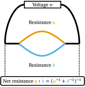
 can be extended to all nonnegative numbers
 ![\[a:h \coloneqq \lim_{b\downarrow a, \: k\downarrow h} b:k = \begin{cases}\left( a^{-1}+h^{-1}\right)^{-1}, & a,h > 0 ,\\0, & \textrm{otherwise}.\end{cases}\]](https://www.ethanepperly.com/wp-content/ql-cache/quicklatex.com-7c49cbcbcd8d8f75fa4f18a40562e718_l3.png "Rendered by QuickLaTeX.com")
 ) if either of the wires carries zero resistance.
![\[A:H = (A^{-1}+H^{-1})^{-1} \quad \text{for $A,H$ positive definite.}\]](https://www.ethanepperly.com/wp-content/ql-cache/quicklatex.com-95cd7707ba37e3436926c73895d537bb_l3.png "Rendered by QuickLaTeX.com")
![\[a:h = \frac{1}{a^{-1}+h^{-1}} = \frac{ah}{a+h} = \frac{a(a+h)-a^2}{a+h} = a - a(a+h)^{-1}a.\]](https://www.ethanepperly.com/wp-content/ql-cache/quicklatex.com-e4e355840ccdeb857cec59c1173cca5b_l3.png "Rendered by QuickLaTeX.com")
![\[A : H = A - A(A+H)^\dagger A.\]](https://www.ethanepperly.com/wp-content/ql-cache/quicklatex.com-85f7337339efbd593339ed3a5ff7e547_l3.png "Rendered by QuickLaTeX.com")
 ,
, for positive definite matrices,
 and
and  .
. is
is  is
is  .
. .
. be the unitarily invariant norm
 ![\begin{align*}\left\|A:H\right\|_{\rm UI} &= \max_{M\succeq 0,\: \left\|M\right\|_{\rm UI}'\le 1} \tr((A:H)M) \\&= \max_{M\succeq 0,\: \left\|M\right\|_{\rm UI}'\le 1} \tr(M^{1/2}(A:H)M^{1/2})\\&= \max_{M\succeq 0,\: \left\|M\right\|_{\rm UI}'\le 1} \tr((M^{1/2}AM^{1/2}):(M^{1/2}HM^{1/2})) \\&\le \max_{M\succeq 0,\: \left\|M\right\|_{\rm UI}'\le 1} \left[\tr(M^{1/2}AM^{1/2}):\tr(M^{1/2}HM^{1/2}) \right] \\&\le \left[\max_{M\succeq 0,\: \left\|M\right\|_{\rm UI}'\le 1} \tr(M^{1/2}AM^{1/2})\right]:\left[\max_{M\succeq 0,\: \left\|M\right\|_{\rm UI}'\le 1} \tr(M^{1/2}HM^{1/2})\right]\\&= \left\|A\right\|_{\rm UI} : \left\|H\right\|_{\rm UI}.\end{align*}](https://www.ethanepperly.com/wp-content/ql-cache/quicklatex.com-4d5c2226a0ddf81d346da401ff4b53b9_l3.png "Rendered by QuickLaTeX.com")
 , the third line is property 6, the fourth line is property 7, the fifth line is property 4, and the sixth line is duality.
![\begin{align*}\left\|B - X\right\|_{\rm Q}^2&\le \left\| \Sigma_2 \right\|_{\rm Q}^2 + \left\|\Sigma_1^2 : [(\Sigma_2\Omega_2\Omega_1^\dagger)^*(\Sigma_2\Omega_2\Omega_1^\dagger)]\right\|_{\rm UI} \\&\le \left\| \Sigma_2 \right\|_{\rm Q}^2 + \left\|\Sigma_1^2\right\|_{\rm UI} : \left\|[(\Sigma_2\Omega_2\Omega_1^\dagger)^*(\Sigma_2\Omega_2\Omega_1^\dagger)]\right\|_{\rm UI} \\&= \left\| \Sigma_2 \right\|_{\rm Q}^2 + \left\|\Sigma_1\right\|_{\rm Q}^2 : \left\|\Sigma_2\Omega_2\Omega_1^\dagger\right\|^2_{\rm Q}.\end{align*}](https://www.ethanepperly.com/wp-content/ql-cache/quicklatex.com-df07b0b9660af51129fd29552ad6c650_l3.png "Rendered by QuickLaTeX.com")
 , we obtain the following expression for the expected error of the randomized SVD
![\[\mathbb{E} \left\|B - X\right\|_{\rm F}^2\le \left\| B - \lowrank{B\right\|_r }_{\rm F}^2 + \mathbb{E}\left\|\Sigma_2\Omega_2\Omega_1^\dagger\right\|^2_{\rm F}. \]](https://www.ethanepperly.com/wp-content/ql-cache/quicklatex.com-3f9645663663b82d968efe393fc4c158_l3.png "Rendered by QuickLaTeX.com")
 . Remarkably, this can be done in closed form.
 and
and  be independent standard Gaussian random matrices with
  ,
,  . Then
![\[\mathbb{E} \left\|SG\Gamma^\dagger R\right\|_{\rm F}^2 = \frac{1}{k-(r+1)}\left\|S\right\|_{\rm F}^2\left\|R\right\|_{\rm F}^2.\]](https://www.ethanepperly.com/wp-content/ql-cache/quicklatex.com-83f5771c01f2d031fd755830d363cda0_l3.png "Rendered by QuickLaTeX.com")
 does not appear:
![\[\mathbb{E} \left\|SGW\right\|_{\rm F}^2 = \mathbb{E} \sum_{ij} \left(\sum_{k\ell} s_{ik}g_{k\ell}w_{\ell j} \right)^2 = \mathbb{E} \sum_{ijk\ell} s_{ik}^2 w_{\ell j}^2 = \left\|S\right\|_{\rm F}^2\left\|W\right\|_{\rm F}^2.\]](https://www.ethanepperly.com/wp-content/ql-cache/quicklatex.com-dc219fd0dab2748965ecbf439c051db5_l3.png "Rendered by QuickLaTeX.com")
 are independent, mean-zero, and variance-one. Thus, applying this result conditionally on
  , we get
![\[\mathbb{E} \left\|SG\Gamma^\dagger R\right\|_{\rm F}^2 =\mathbb{E}\left[ \mathbb{E}\left[ \left\|SG\Gamma^\dagger R\right\|_{\rm F}^2 \,\middle|\, \Gamma\right]\right] =\left\|S\right\|_{\rm F}^2\cdot \mathbb{E} \left\|\Gamma^\dagger R\right\|_{\rm F}^2. \]](https://www.ethanepperly.com/wp-content/ql-cache/quicklatex.com-31c52f341c1e50d4e2c2e8583f3a7737_l3.png "Rendered by QuickLaTeX.com")
 , we rewrite using the
 ![\[\mathbb{E} \left\|\Gamma^\dagger R\right\|_{\rm F}^2 = \mathbb{E} \tr \left(\Gamma^\dagger RR^* \Gamma^{*\dagger} \right)= \tr \left(RR^* \mathbb{E}[\Gamma^{*\dagger}\Gamma^\dagger] \right) = \tr \left(RR^* \mathbb{E}[(\Gamma\Gamma^*)^{-1}] \right).\]](https://www.ethanepperly.com/wp-content/ql-cache/quicklatex.com-79bd47bd70f2015a46c038c4f0d0e5f7_l3.png "Rendered by QuickLaTeX.com")
 is known as an
  . Thus, we obtain
![\[\mathbb{E} \left\|\Gamma^\dagger R\right\|_{\rm F}^2 = \tr \left(RR^* \mathbb{E}[(\Gamma\Gamma^*)^{-1}] \right) = \frac{\tr \left(RR^* \right)}{k-(r+1)} = \frac{\left\|R\right\|_{\rm F}^2}{k-(r+1)}.\]](https://www.ethanepperly.com/wp-content/ql-cache/quicklatex.com-e874bd74b5ef81c13856de05454ea647_l3.png "Rendered by QuickLaTeX.com")
![\[\mathbb{E} \left\|SG\Gamma^\dagger R\right\|_{\rm F}^2 =\left\|S\right\|_{\rm F}^2\cdot \mathbb{E} \left\|\Gamma^\dagger R\right\|_{\rm F}^2 = \frac{1}{k-(r+1)}\left\|S\right\|_{\rm F}^2\left\|R\right\|_{\rm F}^2.\]](https://www.ethanepperly.com/wp-content/ql-cache/quicklatex.com-b2ac63d48bafba095409bc148beed39c_l3.png "Rendered by QuickLaTeX.com")
 are independent and standard Gaussian as well. Plugging the matrix expectation bound to (9) then completes the analysis
 matrix
 ![\[B \approx X \coloneqq Q C.\]](https://www.ethanepperly.com/wp-content/ql-cache/quicklatex.com-c5eb6a2bd93f7c628f485bd473e8676c_l3.png "Rendered by QuickLaTeX.com")
 where
where  and
and  and
and  and
and  .
.![\[B \approx X = QC = U\Sigma V^*.\]](https://www.ethanepperly.com/wp-content/ql-cache/quicklatex.com-8f7c31a46a04e9f0447ddc9209f26458_l3.png "Rendered by QuickLaTeX.com")
 as estimates of the
  numbers of storage, whereas
  numbers of storage. As I detailed at length in my blog post on
  in roughly
  . For these use cases, we don’t need the “SVD” part of the randomized SVD.
 to the matrix
  is than
  .
.![\[\mathbb{E} \left\|B - X\right\|_{\rm F}^2 \le \min_{r \le k-2} \left( 1 + \frac{r}{k-(r+1)} \right) \left\|B - \lowrank{B}_r\right\|^2_{\rm F}. \]](https://www.ethanepperly.com/wp-content/ql-cache/quicklatex.com-aa4c5d7163bac127432706a279ae7210_l3.png "Rendered by QuickLaTeX.com")
 , we see that the randomized SVD error is at most
  times the best rank-
![\[\mathbb{E} \left\|B - X\right\|_{\rm F}^2 \le (1+r) \left\|B - \lowrank{B}_r \right\|^2_{\rm F} \quad \text{for $k=r+2$}. \]](https://www.ethanepperly.com/wp-content/ql-cache/quicklatex.com-29753ca17ed5f7def9297cf52157afb8_l3.png "Rendered by QuickLaTeX.com")
 , we see that the randomized SVD has at most twice the error of the best rank-
![\[\mathbb{E} \left\|B - X\right\|_{\rm F}^2 \le 2 \left\|B - \lowrank{B}_r\right\|^2_{\rm F} \quad \text{for $k=2r+1$}. \]](https://www.ethanepperly.com/wp-content/ql-cache/quicklatex.com-1c11cf4647747653a356178b65c3585f_l3.png "Rendered by QuickLaTeX.com")
 for the randomized SVD suffices. These results hold even for worst-case matrices. For nice matrices with steadily decaying singular values, the randomized SVD can perform even better than equations (2)–(3) would suggest.
![\[\mathbb{E} \left\|B - X\right\|^2 \le \min_{r \le k-2} \left( 1 + \frac{2r}{k-(r+1)} \right) \left(\left\|B - \lowrank{B}_r \right\|^2 + \frac{\mathrm{e}^2}{k-r} \left\|B - \lowrank{B}_r\right\|^2_{\rm F} \right). \]](https://www.ethanepperly.com/wp-content/ql-cache/quicklatex.com-8ee6f467b55a9e949f3636deca2589a5_l3.png "Rendered by QuickLaTeX.com")
![\[\norm{B} = \sigma_1(B),\quad \left\|B\right\|_{\rm F}^2 = \sum_i \sigma_i(B)^2.\]](https://www.ethanepperly.com/wp-content/ql-cache/quicklatex.com-2d3f6deda657f9f0f863a05450571e23_l3.png "Rendered by QuickLaTeX.com")
![\[\mathbb{E} \left\|B - X\right\|^2 \le \min_{r \le k-2} \left( 1 + \frac{2r}{k-(r+1)} \right) \left(\sigma_{r+1}^2 + \frac{\mathrm{e}^2}{k-r} \sum_{i>r} \sigma_i^2 \right).\]](https://www.ethanepperly.com/wp-content/ql-cache/quicklatex.com-d4bb8b98ee0928e647c7cdbd91332fcc_l3.png "Rendered by QuickLaTeX.com")
 , this bound demonstrates that the randomized SVD incurs errors based on the entire tail of
  . The randomized SVD is much worse than the best rank-
 . Powering has the effect of amplifying the large singular values of
  we compute the block
 ![\[B\Omega, BB^*B\Omega, BB^*BB^*B\Omega,\ldots,B(B^*B)^q\Omega\]](https://www.ethanepperly.com/wp-content/ql-cache/quicklatex.com-2584aa789abb8f623fbbb14e114a5461_l3.png "Rendered by QuickLaTeX.com")
![\[Y = \begin{bmatrix} B\Omega & BB^*B\Omega & BB^*BB^*B\Omega& \cdots & B(B^*B)^q\Omega\end{bmatrix}.\]](https://www.ethanepperly.com/wp-content/ql-cache/quicklatex.com-4139403e46250e757c4b558a38b9fba7_l3.png "Rendered by QuickLaTeX.com")
 to obtain accurate results.
 positive semidefinite (psd) matrix
 ![\[\hat{A} = A(:,S) \, A(S,S)^{-1} \, A(S,:), \]](https://www.ethanepperly.com/wp-content/ql-cache/quicklatex.com-cf768b8c5fedfd543a62070abae10bfe_l3.png "Rendered by QuickLaTeX.com")
 identifies a subset of
  , this allowed us to approximate all
  entries of the matrix
  entries in columns
  , where
  is a vector of length
  . The standard way of doing this in modern practice (
 of a lower triangular matrix
  and an upper triangular matrix
  where
where  is a permutation matrix and
  for
for  and then
  for
for  ; the triangularity of
  . This factorization
  is known as a
  , where
  has been replaced by the
 ![\[A = \twobytwo{A_{11}}{A_{12}}{A_{21}}{A_{22}}. \]](https://www.ethanepperly.com/wp-content/ql-cache/quicklatex.com-24b23cd2ac7afc3e7c6acfb7fd8f8220_l3.png "Rendered by QuickLaTeX.com")
 and subtracting this from the second block row introduces a matrix of zeros into the bottom left block of
  is a
is a  for every nonzero vector
 ![\[\twobytwo{I}{0}{-A_{21}A_{11}^{-1}}{I}\twobytwo{A_{11}}{A_{12}}{A_{21}}{A_{22}} = \twobytwo{A_{11}}{A_{12}}{0}{A_{22} - A_{21}A_{11}^{-1}A_{12}}.\]](https://www.ethanepperly.com/wp-content/ql-cache/quicklatex.com-4b8f6deed9a1dd928c76d311ab88fd54_l3.png "Rendered by QuickLaTeX.com")
![\[\twobytwo{I}{0}{-A_{21}A_{11}^{-1}}{I}^{-1} = \twobytwo{I}{0}{A_{21}A_{11}^{-1}}{I}\]](https://www.ethanepperly.com/wp-content/ql-cache/quicklatex.com-be1610a1241e5c5bfd2c7dc04653e712_l3.png "Rendered by QuickLaTeX.com")
![\[A = \twobytwo{A_{11}}{A_{12}}{A_{21}}{A_{22}} = \twobytwo{I}{0}{A_{21}A_{11}^{-1}}{I} \twobytwo{A_{11}}{A_{12}}{0}{A_{22} - A_{21}A_{11}^{-1}A_{12}}.\]](https://www.ethanepperly.com/wp-content/ql-cache/quicklatex.com-e004e13e06bf86fd8707805ce21f9071_l3.png "Rendered by QuickLaTeX.com")
![\[A = \twobytwo{A_{11}}{A_{12}}{A_{21}}{A_{22}} = \twobytwo{I}{0}{A_{21}A_{11}^{-1}}{I} \twobytwo{A_{11}}{0}{0}{A_{22} - A_{21}A_{11}^{-1}A_{12}} \twobytwo{I}{0}{A_{21}A_{11}^{-1}}{I}^*. \]](https://www.ethanepperly.com/wp-content/ql-cache/quicklatex.com-7e3a03d3b1e4421e71d17e2abba7ef97_l3.png "Rendered by QuickLaTeX.com")
 , where
  is a block diagonal matrix.
![\[S = A_{22} - A_{21}A_{11}^{-1}A_{12}. \]](https://www.ethanepperly.com/wp-content/ql-cache/quicklatex.com-55e08632ed61d20591817565b66a7e09_l3.png "Rendered by QuickLaTeX.com")
 in matrix theory makes it deserving of its special name, the Schur complement. To us for now, the Schur complement is just the matrix appearing in the bottom right corner of our block Cholesky factorization.
 is positive (semi)definite, then the Schur complement
  is positive (semi)definite.
 matrix
  .
.![\[A_{11} = L_{11}^{\vphantom{*}}L_{11}^*, \quad S = L_{22}^{\vphantom{*}}L_{22}^*.\]](https://www.ethanepperly.com/wp-content/ql-cache/quicklatex.com-fcde81f118ea8516883b47d07a35b2b0_l3.png "Rendered by QuickLaTeX.com")
 factorization (1) and simplifying gives a Cholesky factorization, as desired:
![\[A = \twobytwo{L_{11}}{0}{A_{21}^{\vphantom{*}}(L_{11}^{*})^{-1}}{L_{22}}\twobytwo{L_{11}}{0}{A_{21}^{\vphantom{*}}(L_{11}^{*})^{-1}}{L_{22}}^* =: LL^*.\]](https://www.ethanepperly.com/wp-content/ql-cache/quicklatex.com-e22f8c5665f2154819e960cd6c6b32d3_l3.png "Rendered by QuickLaTeX.com")
 , perform the following steps:
 th column of
 ![\[L(j:N,j) \leftarrow A(j:N,j)/\sqrt{a_{jj}}.\]](https://www.ethanepperly.com/wp-content/ql-cache/quicklatex.com-9d8a1752f0ae4613f71767ce87b9560a_l3.png "Rendered by QuickLaTeX.com")
![\[A(j+1:N,j+1:N)\leftarrow A(j+1:N,j+1:N) - \frac{A(j+1:N,j)A(j,j+1:N)}{a_{jj}}.\]](https://www.ethanepperly.com/wp-content/ql-cache/quicklatex.com-d8090111efb4d1beb891cac29c04a598_l3.png "Rendered by QuickLaTeX.com")
![\[A = \twobytwo{I}{0}{A_{21}A_{11}^{-1}}{I} \twobytwo{A_{11}}{0}{0}{A_{22} - A_{21}A_{11}^{-1}A_{12}} \twobytwo{I}{0}{A_{21}A_{11}^{-1}}{I}^*.\]](https://www.ethanepperly.com/wp-content/ql-cache/quicklatex.com-7d369f0415a2b62af274f183e8828853_l3.png "Rendered by QuickLaTeX.com")
 , which is a large matrix of size
  .
.![\[A = \twobyone{I}{A_{21}{A_{11}^{-1}}} A_{11} \twobyone{I}{A_{22}{A_{11}^{-1}}}^* + \twobytwo{0}{0}{0}{A_{22}-A_{21}A_{11}^{-1}A_{12}}. \]](https://www.ethanepperly.com/wp-content/ql-cache/quicklatex.com-eb7264120d2157941336da3dcbbcc1d8_l3.png "Rendered by QuickLaTeX.com")
![\[\hat{A} = \twobyone{A_{11}}{A_{21}} A_{11}^{-1} \onebytwo{A_{11}}{A_{12}} = \twobytwo{A_{11}}{A_{12}}{A_{21}}{A_{21}A_{11}^{-1}A_{12}},\]](https://www.ethanepperly.com/wp-content/ql-cache/quicklatex.com-8ec34b04edefd156d8de3711608998b2_l3.png "Rendered by QuickLaTeX.com")
 and is the final of our three titular characters. The residual of the Nyström approximation is the second term in (2), which is none other than the Schur complement (Sch), padded by rows and columns of zeros:
![\[A - \hat{A} = \twobytwo{0}{0}{0}{A_{22}-A_{21}A_{11}^{-1}A_{12}}.\]](https://www.ethanepperly.com/wp-content/ql-cache/quicklatex.com-f8dccb2f8fd446335886ec9bdabc85da_l3.png "Rendered by QuickLaTeX.com")
 followed by position
  and so on. There’s no need to insist on this exact ordering of elimination steps. Indeed, at each step of the Cholesky algorithm, we can choose whichever diagonal position
  that we want to perform elimination. The entry we choose to perform elimination with is called a
  matrix
  , in factored form. For
  , perform the following steps:
 .
. .
. .
.![\[\hat{A} = FF^* = A(:,S) \, A(S,S)^{-1} \, A(S,:).\]](https://www.ethanepperly.com/wp-content/ql-cache/quicklatex.com-f9ac31fa249d889cd909be1d340abd58_l3.png "Rendered by QuickLaTeX.com")
![\[s_j = \argmax_{1\le k\le N} a_{kk}.\]](https://www.ethanepperly.com/wp-content/ql-cache/quicklatex.com-42a58dd2bd6824be5efdc930fc5356df_l3.png "Rendered by QuickLaTeX.com")
![\[\mathbb{P} \{ s_j = k \} = \frac{a_{kk}}{\operatorname{tr} A}.\]](https://www.ethanepperly.com/wp-content/ql-cache/quicklatex.com-36ca3921c45ffb034e0cfa8adf85b982_l3.png "Rendered by QuickLaTeX.com")
![\[A\langle \Omega\rangle := A\Omega \, (\Omega^*A\Omega)^{-1} \, \Omega^*A. \]](https://www.ethanepperly.com/wp-content/ql-cache/quicklatex.com-636eb074d4ce2e59defede1f1be7877d_l3.png "Rendered by QuickLaTeX.com")
 is invertible; if
  is invertible in this post, though everything we discuss will continue to work if this assumption is dropped. I use
  .
. , we observe that the Nyström approximation can be written entirely using
 ![\[A\langle \Omega\rangle = Y \, (\Omega^* Y)^{-1}\, Y^*.\]](https://www.ethanepperly.com/wp-content/ql-cache/quicklatex.com-4332839cf045146208c9b58c395aefc4_l3.png "Rendered by QuickLaTeX.com")
 is only rank at most
  to be closer to the eigenvectors of
  of the identity matrix, then
  of
of ![\[A(:,\{i_1,\ldots,i_k\}) = A\Omega \quad \text{for}\quad \Omega = I(:,\{i_1,i_2,\ldots,i_k\}).\]](https://www.ethanepperly.com/wp-content/ql-cache/quicklatex.com-49181e8e724ecddcd4646eb90f3bc35e_l3.png "Rendered by QuickLaTeX.com")
 . As a first step, we shall show that the residual is psd. This means that
 ![\[A\langle \Omega \rangle = A^{1/2} P_{A^{1/2}\Omega} A^{1/2}.\]](https://www.ethanepperly.com/wp-content/ql-cache/quicklatex.com-4cc583dbaca6e6da9c53ad3327717346_l3.png "Rendered by QuickLaTeX.com")
 denotes the the
  . To deduce the projection formula, we break down
  in (1):
![\[A\langle \Omega\rangle = A^{1/2} \left( A^{1/2}\Omega \left[ (A^{1/2}\Omega)^* A^{1/2}\Omega \right]^{-1} (A^{1/2}\Omega)^* \right) A^{1/2}.\]](https://www.ethanepperly.com/wp-content/ql-cache/quicklatex.com-2880bf8a43ee68664131becfdc0b3d19_l3.png "Rendered by QuickLaTeX.com")
 , where
  . The parenthesized expression is
  .
.![\[A - A\langle \Omega\rangle = A^{1/2} (I - P_{A^{1/2}\Omega}) A^{1/2}.\]](https://www.ethanepperly.com/wp-content/ql-cache/quicklatex.com-23f5459646b6b93d24c7e107f636a3d5_l3.png "Rendered by QuickLaTeX.com")
 is psd. If
  is an orthogonal projection and therefore psd. Thus, by the conjugation rule, the residual of the is Nyström approximation is psd:
![\[A - A\langle \Omega\rangle = \left(A^{1/2}\right)^* (I-P_{A^{1/2}\Omega})A^{1/2} \quad \text{is psd}.\]](https://www.ethanepperly.com/wp-content/ql-cache/quicklatex.com-a06ad324c77c1acb2f4563bff24686a7_l3.png "Rendered by QuickLaTeX.com")
![\[\left\|UBV\right\|_{\rm UI} = \left\|B\right\|_{\rm UI} \quad \text{for all unitary matrices $U$ and $V$.}\]](https://www.ethanepperly.com/wp-content/ql-cache/quicklatex.com-e3f67a9a35ce0ba62f155eb0cddcf1f2_l3.png "Rendered by QuickLaTeX.com")
 . Unitary matrices preserve the
  . For instance, the spectral, Frobenius, and nuclear norms take the forms
 , then
  for every unitarily invariant norm
  , if the difference
  is psd. As a consequence,
  if and only if
  .
. , it seems natural to expect that
  for every unitarily invariant norm
 ![\[\hat{A} = A\Omega \, T \, (A\Omega)^* = A \Omega \, T \, \Omega^*A,\]](https://www.ethanepperly.com/wp-content/ql-cache/quicklatex.com-0955f7609913774307be45326f9a1dfd_l3.png "Rendered by QuickLaTeX.com")
 is a self-adjoint matrix. To make this more similar to the projection formula, we can factor
 ![\[\hat{A} = A^{1/2} (A^{1/2}\Omega\, T\, \Omega^*A^{1/2}) A^{1/2}.\]](https://www.ethanepperly.com/wp-content/ql-cache/quicklatex.com-6e53f93f84078b4f7a0c921ee5bb6e8d_l3.png "Rendered by QuickLaTeX.com")
![\[\hat{A} = A^{1/2} \,QMQ^*\, A^{1/2} \quad \text{where} \quad M\text{ is self-adjoint}.\]](https://www.ethanepperly.com/wp-content/ql-cache/quicklatex.com-59f6b786fcfd454b3e037d9cfd0a5b50_l3.png "Rendered by QuickLaTeX.com")
![\[A - \hat{A} = A^{1/2} (I - QMQ^*)A^{1/2}. \]](https://www.ethanepperly.com/wp-content/ql-cache/quicklatex.com-d8a588c5112e24aba21783fd38c417b8_l3.png "Rendered by QuickLaTeX.com")
 is psd (property 3), the conjugation rule tells us that
![\[I - QMQ^*\succeq 0.\]](https://www.ethanepperly.com/wp-content/ql-cache/quicklatex.com-f5f4a27c026c6cb4a5c756cf9bfea0ac_l3.png "Rendered by QuickLaTeX.com")
 ? We can apply the conjugation rule again to conclude
![\[Q^*(I - QMQ^*)Q = Q^*Q - (Q^*Q)M(Q^*Q) = I-M \succeq 0.\]](https://www.ethanepperly.com/wp-content/ql-cache/quicklatex.com-835a14c1d767ffd164f996bffd8b4de5_l3.png "Rendered by QuickLaTeX.com")
 since
since  . Indeed,
 and the last line is the conjugation rule combined with the fact that
  is psd. Thus, having shown
![\[A - \hat{A} \succeq A - A\langle\Omega\rangle \succeq 0,\]](https://www.ethanepperly.com/wp-content/ql-cache/quicklatex.com-3617754c93689afb140dcd12ad0b7e80_l3.png "Rendered by QuickLaTeX.com")
![\[\|A - \hat{A}\|_{\rm UI} \ge \left\|A - A\langle \Omega\rangle\right\|_{\rm UI} \quad \text{for every unitarily invariant norm $\left\|\cdot\right\|_{\rm UI}$}.\]](https://www.ethanepperly.com/wp-content/ql-cache/quicklatex.com-c89ba0ba57313ce5f778324faf3bff2f_l3.png "Rendered by QuickLaTeX.com")