This post is co-written by my brother, Aidan Epperly, for the second Summer of Math Exposition (SoME2).
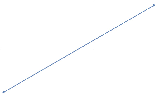
Let’s start with a classical problem: connect-the-dots. As we know from geometry, any two points in the plane are connected by one and only one straight line:
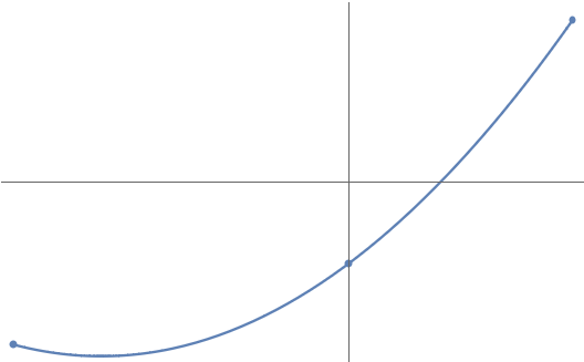
But what if we have more than two points? How should we connect them? One natural way is by parabola. Any three points (with distinct  coordinates) are connected by one and only one parabola
  :
:
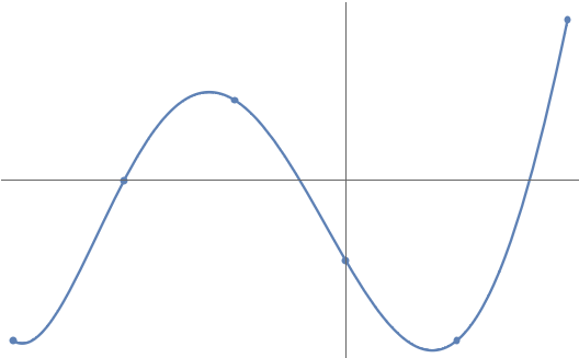
And we can keep extending this. Any  points1The degree of the polynomial is one less than the number of points because a degree-
 polynomial is described by coefficients. For instance, a degree-two parabola has three coefficients
  ,
,  , and
, and  . (with distinct coordinates) are connected by a unique degree- polynomial
  :
:
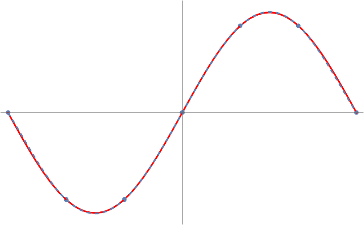
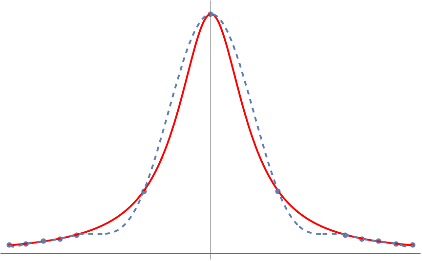
This game of connect-the-dots with polynomials is known more formally as polynomial interpolation. We can use polynomial interpolation to approximate functions. For instance, we can approximate the function  on the interval
 ![[-\pi,\pi]](https://www.ethanepperly.com/wp-content/ql-cache/quicklatex.com-db4571552bede65e472ffbfee6887855_l3.png "Rendered by QuickLaTeX.com") to visually near-perfect accuracy by connecting the dots between seven points
to visually near-perfect accuracy by connecting the dots between seven points  :
:
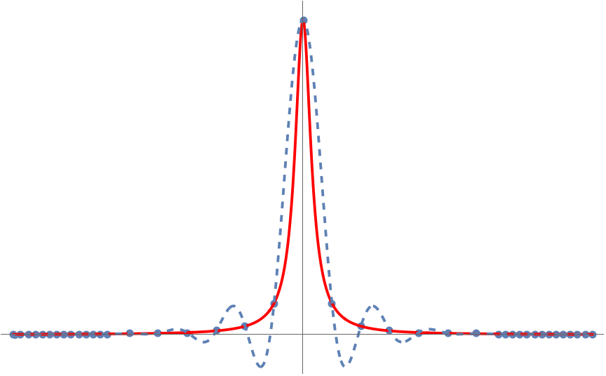
But something very peculiar happens when we try and apply this trick to the specially chosen function  on the interval
 ![[-1,1]](https://www.ethanepperly.com/wp-content/ql-cache/quicklatex.com-634fe4705a526f221e312cffd3ceda93_l3.png "Rendered by QuickLaTeX.com") :
:
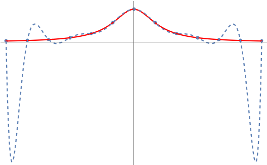
Unlike , the polynomial interpolant for  is terrible! What’s going on? Why doesn’t polynomial interpolation work here? Can we fix it? The answer to the last question is yes and the solution is Chebyshev polynomials.
Reverse-Engineering Chebyshev
The failure of polynomial interpolation for is known as Runge’s phenomenon after Carl Runge who discovered this curious behavior in 1901. The function is called the Runge function. Our goal is to find a fix for polynomial interpolation which crushes the Runge phenomenon, allowing us to reliably approximate every sensible2A famous theorem of Faber states that there does not exist any set of points through which the polynomial interpolants converge for every continuous function. This is not as much of a problem as it may seem. As the famous Weierstrass function shows, arbitrary continuous functions can be very weird. If we restrict ourselves to nicer functions, such as Lipschitz continuous functions, there does exist a set of points through which the polynomial interpolant always converges to the underlying function. Thus, in this senses, it is possible to crush the Runge phenomenon. function with polynomial interpolation.
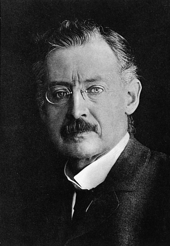
Carl Runge
Let’s put on our thinking caps and see if we can discover the fix for ourselves. In order to discover a fix, we must first identify the problem. Observe that the polynomial interpolant is fine near the center of the interval; it only fails near the boundary.

This leads us to a guess for what the problem might be; maybe we need more interpolation points near the boundaries of the interval. Indeed, tipping our hand a little bit, this turns out to be the case. For instance, connecting the dots for the following set of “mystery points” clustered at the endpoints works just fine:
Let’s experiment a little and see if we can discover a nice set of interpolation points, which we will call  , like this for ourselves. We’ll assume the interpolation points are given by a function
  so we can form the polynomial interpolant for any desired polynomial degree .3Technically, we should insist on the function
  being \textit{injective} so that the points
  are guaranteed to be distinct. For instance, if we pick
  , the points look like this:
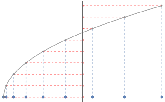
Equally spaced points  (shown on vertical axis) give rise to
non-equally spaced points  (shown on horizontal axis)
How should we pick the function ? First observe that, even for the Runge function, equally spaced interpolation points are fine near the center of the interval. We thus have at least two conditions for our desired interpolation points:
- The interior points should maintain their spacing of roughly
 .
. - The points must cluster near both boundaries.
As a first attempt let’s divide the interval into thirds and halve the spacing of points except in the middle third. This leads to the function

These interpolation points initially seem promising, even successfully approximating the Runge function itself.
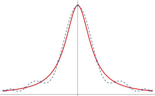
Unfortunately, this set of points fails when we consider other functions. For instance, if we use the Runge-like function  , we see that these interpolation points now lead to a failure to approximate the function at the middle of the interval, even if we use a lot of interpolation points!
Maybe the reason this set of interpolation points didn’t work is that the points are too close at the endpoints. Or maybe we should have divided the interval as quarter–half–quarter rather than thirds. There are lots of variations of this strategy for choosing points to explore and all of them eventually lead to failure on some Runge-flavored example. We need a fundamentally different strategy then making the points times closer within distance of the endpoints.
Let’s try a different approach. The closeness of the points at the endpoints is determined by the slope of the function  at
at  and
and  . The smaller that
  and
and  are, the more clustered the points will be. For instance,

When we halved the distance between points, we instead had

So if we want the points to be much more clustered together, it is natural to require

It also makes sense for the function to cluster points equally near both endpoints, since we see no reason to preference one end over the other. Collecting together all the properties we want the function to have, we get the following list:
- spans the whole range ,
 , and
, and- is symmetric about
 ,
,  .
.
Mentally scrolling through our Rolodex of friendly functions, a natural one that might come to mind meeting these three criteria is the cosine function, specifically  . This function yields points which are more clustered at the endpoints:

The points

we guessed our way into are known as the Chebyshev points.4Some authors refer to these as the “Chebyshev points of the second kind” or use other names. We follow the convention in Approximation Theory and Approximation Practice (Chapter 1) and simply refer to these points simply as the Chebyshev points. The Chebyshev points prove themselves perfectly fine for the Runge function:

As we saw earlier, success on the Runge function alone is not enough to declare victory for the polynomial interpolation problem. However, in this case, there are no other bad examples left to find. For any nice function with no jumps, polynomial interpolation through the Chebyshev points works excellently.5Specifically, for a function  which not too rough (i.e., Lipschitz continuous), the degree- polynomial interpolant of through the Chevyshev points converges uniformly to as
  .
.
Why the Chebyshev Points?
We’ve guessed our way into a solution to the polynomial interpolation problem, but we still really don’t know what’s going on here. Why are the Chebyshev points much better at polynomial interpolation than equally spaced ones?
Now that we know that the Chebyshev points are a right answer to the interpolation problem,6Indeed, there are other sets of interpolation points through which polynomial interpolation also works well, such as the Legendre points. let’s try and reverse engineer a principled reason for why we would expect them to be effective for this problem. To do this, we ask:
What is special about the cosine function?
From high school trigonometry, we know that  gives the coordinate of a point
  radians along the unit circle. This means that the Chebyshev points are the coordinates of equally spaced points on the unit circle (specifically the top half of the unit circle
  ).
).
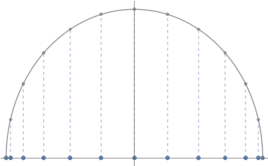
Chebyshev points are the coordinates of equally spaced points on the unit circle.
This raises the question:
What does the interpolating polynomial  look like as a function of the angle ?
To convert between and we simply plug in  to :
to :

This new function depending on , which we can call  , is a polynomial in the variable . Powers of cosines are not something we encounter every day, so it makes sense to try and simplify things using some trig identities. Here are the first couple powers of cosines:

A pattern has appeared! The powers  always take the form7As a fun exercise, you might want to try and prove this using mathematical induction.

The significance of this finding is that, by plugging in each of these formulas for , we see that our polynomial in the variable has morphed into a Fourier cosine series in the variable :

For anyone unfamiliar with Fourier series, we highly encourage the 3Blue1Brown video on the subject, which explains why Fourier series are both mathematically beautiful and practically useful. The basic idea is that almost any function can be expressed as a combination of waves (that is, sines and cosines) with different frequencies.8More precisely, we might call these angular frequencies. In our case, this formula tells us that is equal to  units of frequency , plus
  units of frequency , all the way up to
  units of frequency . Different types of Fourier series are appropriate in different contexts. Since our Fourier series only possesses cosines, we call it a Fourier cosine series.
We’ve discovered something incredibly cool:
Polynomial interpolation through the Chebyshev points is equivalent to finding a Fourier cosine series for equally spaced angles
We’ve arrived at an answer to why the Chebyshev points work well for polynomial interpolation.
Polynomial interpolation through the Chebyshev points is effective because Fourier cosine series through equally spaced angles
Of course, this explanation just raises the further question: Why do Fourier cosine series give effective interpolants through equally spaced angles ? This question has a natural answer as well, involving the convergence theory and aliasing formula (see Section 3 of this paper) for Fourier series. We’ll leave the details to the interested reader for investigation. The success of Fourier cosines series in interpolating equally spaced data is a fundamental observation that underlies the field of digital signal processing. Interpolation through the Chebyshev points effectively hijacks this useful fact and applies it to the seemingly unrelated problem of polynomial interpolation.
Another question this explanation raises is the precise meaning of “effective”. Just how good are polynomial interpolants through the Chebyshev points at approximating functions? As is discussed at length in another post on this blog, the degree to which a function can be effectively approximated is tied to how smooth or rough it is. Chebyshev interpolants approximate nice analytic functions like or  with exponentially small errors in the number of interpolation points used. By contrast, functions with kinks like
  are approximated with errors which decay much more slowly. See theorems 2 and 3 on this webpage for more details.
Chebyshev Polynomials
We’ve now discovered a set of points, the Chebyshev points, through which polynomial interpolation works well. But how should we actually compute the interpolating polynomial

Again, it will be helpful to draw on the connection to Fourier series. Computations with Fourier series are highly accurate and can be made lightning fast using the fast Fourier transform algorithm. By comparison, directly computing with a polynomial through its coefficients  is a computational nightmare.
In the variable , the interpolant takes the form
To convert back to , we use the inverse function9One always has to be careful when going from to  since multiple values get mapped to a single value by the cosine function. Fortunately, we’re working with variables and
  , between which the cosine function is one-to-one with the inverse function being given by the arccosine. to obtain:

This is a striking formula. Given all of the trigonometric functions, it’s not even obvious that is a polynomial (it is)!
Despite its seeming peculiarity, this is a very powerful way of representing the polynomial . Rather than expressing using monomials  , we’ve instead written as a combination of more exotic polynomials

The polynomials  are known as the Chebyshev polynomials,10More precisely, the polynomials
  are known as the Chebyshev polynomials of the first kind. named after Pafnuty Chebyshev who studied the polynomials intensely.11The letter “T” is used for Chebyshev polynomials since the Russian name “Chebyshev” is often alternately transliterated to English as “Tchebychev”.
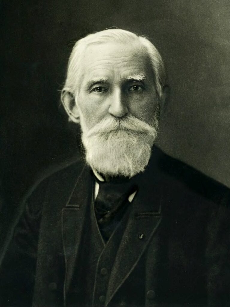
Pafnuty Chebyshev
Writing out the first few Chebyshev polynomials shows they are indeed polynomials:

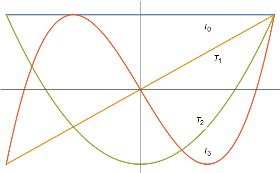
The first four Chebyshev polynomials
To confirm that this pattern does continue, we can use trig identities to derive12Specifically, the recurrence is a consequence of applying the sum-to-product identity to  for . the following recurrence relation for the Chebyshev polynomials:

Since  and
and  are both polynomials, every Chebyshev polynomial is as well.
We’ve arrived at the following amazing conclusion:
Under the change of variables
becomes the combination of Chebyshev polynomials
![\[p^\circ(\theta) = b_n\cos(n\theta) + \cdots + b_1\cos\theta + b_0\]](https://www.ethanepperly.com/wp-content/ql-cache/quicklatex.com-1c6828300bbae5fa0051e7c134da1d61_l3.png "Rendered by QuickLaTeX.com")
![\[p(x) = b_nT_n(x) + \cdots + b_1 T_1(x) + b_0.\]](https://www.ethanepperly.com/wp-content/ql-cache/quicklatex.com-cb291d9f73ebc4e74d0455dac4558a48_l3.png "Rendered by QuickLaTeX.com")
This simple and powerful observations allows us to apply the incredible speed and accuracy of Fourier series to polynomial interpolation.
Beyond being a neat idea with some nice mathematics, this connection between Fourier series and Chebyshev polynomials is a powerful tool for solving computational problems. Once we’ve accurately approximated a function by a polynomial interpolant, many quantities of interest (derivatives, integrals, zeros) become easy to compute—after all, we just have to compute them for a polynomial! We can also use Chebyshev polynomials to solve differential equations with much faster rates of convergence than other methods. Because of the connection to Fourier series, all of these computations can be done to high accuracy and blazingly fast via the fast Fourier transform, as is done in the software package Chebfun.
The Chebyshev polynomials have an array of amazing properties and they appear all over mathematics and its applications in other fields. Indeed, we have only scratched the surface of the surface. Many questions remain:
- What is the connection between the Chebyshev points and the Chebyshev polynomials?
- The cosine functions
 are orthogonal to each other; are the Chebyshev polynomials?
 - Are the Chebyshev points the best points for polynomial interpolation? What does “best” even mean in this context?
- Every “nice” even periodic function has an infinite Fourier cosine series which converges to it. Is there a Chebyshev analog? Is there a relation between the infinite Chebyshev series and the (finite) interpolating polynomial through the Chebyshev points?
All of these questions have beautiful and fairly simple answers. The book Approximation Theory and Approximation Practice is a wonderfully written book that answers all of these questions in its first six chapters, which are freely available on the author’s website. We recommend the book highly to the curious reader.
TL;DR: To get an accurate polynomial approximation, interpolate through the Chebyshev points.
To compute the resulting polynomial, change variables to , compute the Fourier cosine series interpolant, and obtain your polynomial interpolant as a combination of Chebyshev polynomials.
I’m aware those “spike error” in the polynomial interpolation for quite some time. However, I don’t even bother look if there a way to fix it (and just eyeballing w/ trig/expo interpolation instead)!
Thank you!