I am excited to share that our paper XTrace: Making the most of every sample in stochastic trace estimation has been published in the SIAM Journal on Matrix Analysis and Applications. (See also our paper on arXiv.)
Spurred by this exciting news, I wanted to take the opportunity to share one of my favorite results in randomized numerical linear algebra: a “speed limit” result of Meyer, Musco, Musco, and Woodruff that establishes a fundamental limitation on how accurate any trace estimation algorithm can be.
Let’s back up. Given an unknown square matrix  , the trace of , defined to be the sum of its diagonal entries
![\[\tr(A) \coloneqq \sum_{i=1}^n A_{ii}.\]](https://www.ethanepperly.com/wp-content/ql-cache/quicklatex.com-80cd9a9ca29d1d3bb13ce28fd80b5e59_l3.png "Rendered by QuickLaTeX.com")
through matrix–vector products (affectionately known as “matvecs”): Given any vector  , we have access to
  . Our goal is to form an estimate
  that is as accurate as possible while using as few matvecs as we can get away with.
To simplify things, let’s assume the matrix is symmetric and positive (semi)definite. The classical algorithm for trace estimation is due to Girard and Hutchinson, producing a probabilistic estimate with a small average (relative) error:
![\[\expect\left[\frac{|\hat{\tr}-\tr(A)|}{\tr(A)}\right] \le \varepsilon \quad \text{using } m= \frac{\rm const}{\varepsilon^2} \text{ matvecs}.\]](https://www.ethanepperly.com/wp-content/ql-cache/quicklatex.com-07898a8a2214416cb97b8b72956e3e76_l3.png "Rendered by QuickLaTeX.com")
 ) requires roughly
  matvecs!
This state of affairs was greatly improved by Meyer, Musco, Musco, and Woodruff. Building upon previous work, they proposed the Hutch++ algorithm and proved it outputs an estimate satisfying the following bound:
(1) ![\[\expect\left[\frac{|\hat{\tr}-\tr(A)|}{\tr(A)}\right] \le \varepsilon \quad \text{using } m= \frac{\rm const}{\varepsilon} \text{ matvecs}.\]](https://www.ethanepperly.com/wp-content/ql-cache/quicklatex.com-b9f186640222c78e5064f83465038b78_l3.png "Rendered by QuickLaTeX.com")
 matvecs to achieve 1% error! Our algorithm, XTrace, satisfies the same error guarantee (1) as Hutch++. On certain problems, XTrace can be quite a bit more accurate than Hutch++.
The MMMW Trace Estimation “Speed Limit”
Given the dramatic improvement of Hutch++ and XTrace over Girard–Hutchinson, it is natural to hope: Is there an algorithm that does even better than Hutch++ and XTrace? For instance, is there an algorithm satisfying an even slightly better error bound of the form
![\[\expect\left[\frac{|\hat{\tr}-\tr(A)|}{\tr(A)}\right] \le \varepsilon \quad \text{using } m= \frac{\rm const}{\varepsilon^{0.999}} \text{ matvecs}?\]](https://www.ethanepperly.com/wp-content/ql-cache/quicklatex.com-8bae682300a401dc80869764b302ce8c_l3.png "Rendered by QuickLaTeX.com")
Let’s add some fine print. Consider an algorithm for the trace estimation problem. Whenever the algorithm wants, it can present a vector  and receive back
  . The algorithm is allowed to be adaptive: It can use the matvecs
  it has already collected to decide which vector
  to present next. We measure the cost of the algorithm in terms of the number of matvecs alone, and the algorithm knows nothing about the psd matrix other what it learns from matvecs.
One final stipulation:
Simple entries assumption. We assume that the entries of the vectors
and
with up to
digits after the decimal place.
To get a feel for this simple entries assumption, suppose we set  . Then
  would be an allowed input vector, but
  would not be (too many digits after the decimal place). Similarly,
  would not be valid because its entries exceed . The simple entries assumption is reasonable as we typically represent numbers on digital computers by storing a fixed number of digits of accuracy.1We typically represent numbers on digital computers by floating point numbers, which essentially represent numbers using scientific notation like
  . For this analysis of trace estimation, we use fixed point numbers like
  (no powers of ten allowed)!
With all these stipulations, we are ready to state the “speed limit” for trace estimation proved by Meyer, Musco, Musco, and Woodruff:
Informal theorem (Meyer, Musco, Musco, Woodruff). Under the assumptions above, there is no trace estimation algorithm producing an estimate
![\[\expect\left[\frac{|\hat{\tr}-\tr(A)|}{\tr(A)}\right] \le \varepsilon \quad \text{using } m= \frac{\rm const}{\varepsilon^{0.999}} \text{ matvecs}.\]](https://www.ethanepperly.com/wp-content/ql-cache/quicklatex.com-9034edba9bafb68809d24d54f5a830e6_l3.png "Rendered by QuickLaTeX.com")
We will see a slightly sharper version of the theorem below, but this statement captures the essence of the result.
Communication Complexity
To prove the MMMW theorem, we have to take a journey to the beautiful subject of communication complexity. The story is this. Alice and Bob are interested in solving a computational problem together. Alice has her input and Bob has his input  , and they are interested in computing a function
  of both their inputs.
Unfortunately for the two of them, Alice and Bob are separated by a great distance, and can only communicate by sending single bits (0 or 1) of information over a slow network connection. Every bit of communication is costly. The field of communication complexity is dedicated to determining how efficiently Alice and Bob are able to solve problems of this form.
The Gap-Hamming problem is one example of a problem studied in communication complexity. As inputs, Alice and Bob receive vectors  with
with  and entries from a third party Eve. Eve promises Alice and Bob that their vectors and satisfy one of two conditions:
(2) ![\[\text{Case 0: } x^\top y \ge\sqrt{n} \quad \text{or} \quad \text{Case 1: } x^\top y \le -\sqrt{n}. \]](https://www.ethanepperly.com/wp-content/ql-cache/quicklatex.com-3134941eeedf133f83ba4795b499332f_l3.png "Rendered by QuickLaTeX.com")
There’s one simple solution to this problem: First, Bob sends his whole input vector to Alice. Each entry of takes one of the two value  and can therefore be communicated in a single bit. Having received , Alice computes
  , determines whether they are in case 0 or case 1, and sends Bob a single bit to communicate the answer. This procedure requires
  bits of communication.
Can Alice and Bob still solve this problem with many fewer than  bits of communication, say
  bits? Unfortunately not. The following theorem of Chakrabati and Regev shows that roughly bits of communication are needed to solve this problem:
Theorem (Chakrabati–Regev). Any algorithm which solves the Gap-Hamming problem that succeeds with at least
probability for every pair of inputs
bits of communication.
Here, is big-Omega notation, closely related to big-O notation  and big-Theta notation
  . For the less familiar, it can be helpful to interpret , , and as all standing for “proportional to ”. In plain language, the theorem of Chakrabati and Regev result states that there is no algorithm for the Gap-Hamming problem that much more effective than the basic algorithm where Bob sends his whole input to Alice (in the sense of requiring less than bits of communication).
Reducing Gap-Hamming to Trace Estimation
This whole state of affairs is very sad for Alice and Bob, but what does it have to do with trace estimation? Remarkably, we can use hardness of the Gap-Hamming problem to show there’s no algorithm that fundamentally improves on Hutch++ and XTrace. The argument goes something like this:
- If there were a trace estimation algorithm fundamentally better than Hutch++ and XTrace, we could use it to solve Gap-Hamming in fewer than bits of communication.
- But no algorithm can solve Gap-Hamming in fewer than bits or communication.
- Therefore, no trace estimation algorithm is fundamentally better than Hutch++ and XTrace.
Step 2 is the work of Chakrabati and Regev, and step 3 follows logically from 1 and 2. Therefore, we are left to complete step 1 of the argument.
Protocol
Assume we have access to a really good trace estimation algorithm. We will use it to solve the Gap-Hamming problem. For simplicity, assume is a perfect square. The basic idea is this:
- Have Alice and Bob reshape their inputs into matrices
 , and consider (but do not form!) the positive semidefinite matrix
 ![\[A = (X+Y)^\top (X+Y).\]](https://www.ethanepperly.com/wp-content/ql-cache/quicklatex.com-2b1df104e3d571430963573b54d5c4df_l3.png "Rendered by QuickLaTeX.com")
- Observe that
Thus, the two cases in (2) can be equivalently written in terms of![\[\tr(A) = \tr(X^\top X) + 2\tr(X^\top Y) + \tr(Y^\top Y) = 2n + 2(x^\top y).\]](https://www.ethanepperly.com/wp-content/ql-cache/quicklatex.com-a0f6e916740a9c27733c659418cc15cf_l3.png "Rendered by QuickLaTeX.com")
 :
:(2′)
![\[\text{Case 0: } \tr(A)\ge 2n + 2\sqrt{n} \quad \text{or} \quad \text{Case 1: } \tr(A) \le 2n-2\sqrt{n}. \]](https://www.ethanepperly.com/wp-content/ql-cache/quicklatex.com-1fea970636b48c827e4584d3655b9e3c_l3.png "Rendered by QuickLaTeX.com")
- By working together, Alice and Bob can implement a trace estimation algorithm. Alice will be in charge of running the algorithm, but Alice and Bob must work together to compute matvecs. (Details below!)
- Using the output of the trace estimation algorithm, Alice determines whether they are in case 0 or 1 (i.e., where
 or
or  ) and sends the result to Bob.
To complete this procedure, we just need to show how Alice and Bob can implement the matvec procedure using minimal communication. Suppose Alice and Bob want to compute  for some vector
  with entries between and with up to decimal digits. First, convert to a vector
  whose entries are integers between
  and
and  . Since
  , interconverting between and
  is trivial. Alice and Bob’s procedure for computing is as follows:
- Alice sends Bob
 .
. - Having received , Bob forms
 and sends it to Alice.
 - Having received , Alice computes
 and sends it to Bob.
 - Having received
 , Bob computes
  and sends its to Alice.
 - Alice forms
 .
.
Because  and
and  are
are  and have entries, all vectors computed in this procedure are vectors of length with integer entries between
  and
and  . We conclude the communication cost for one matvec is
  bits.
bits.
Analysis
Consider an algorithm we’ll call BestTraceAlgorithm. Given any accuracy parameter  , BestTraceAlgorithm requires at most
  matvecs and, for any positive semidefinite input matrix of any size, produces an estimate satisfying
(3) ![\[\expect\left[\frac{|\hat{\tr}-\tr(A)|}{\tr(A)}\right] \le \varepsilon.\]](https://www.ethanepperly.com/wp-content/ql-cache/quicklatex.com-a9165ea3846d540eb654af9f7f59a5c2_l3.png "Rendered by QuickLaTeX.com")
 matvecs.
To solve the Gap-Hamming problem, Alice and Bob just need enough accuracy in their trace estimation to distinguish between cases 0 and 1. In particular, if
![\[\left| \frac{\hat{\tr} - \tr(A)}{\tr(A)} \right| \le \frac{1}{\sqrt{n}},\]](https://www.ethanepperly.com/wp-content/ql-cache/quicklatex.com-8327e1b03c9ba9162fb737e40a192b3a_l3.png "Rendered by QuickLaTeX.com")
Suppose that Alice and Bob apply trace estimation to solve the Gap-Hamming problem, using  matvecs in total. The total communication is
  bits. Chakrabati and Regev showed that Gap-Hamming requires
  bits of communication (for some
  ) to solve the Gap-Hamming problem with probability. Thus, if
  , then Alice and Bob fail to solve the Gap-Hamming problem with at least
  probability. Thus,
![\[\text{If } m < \frac{cn}{T} = \Theta\left( \frac{\sqrt{n}}{b+\log n} \right), \quad \text{then } \left| \frac{\hat{\tr} - \tr(A)}{\tr(A)} \right| > \frac{1}{\sqrt{n}} \text{ with probability at least } \frac{1}{3}.\]](https://www.ethanepperly.com/wp-content/ql-cache/quicklatex.com-74364fd915239fdaf0889d005378b7ba_l3.png "Rendered by QuickLaTeX.com")
![\[\text{If }\left| \frac{\hat{\tr} - \tr(A)}{\tr(A)} \right| \le \frac{1}{\sqrt{n}}\text{ with probability at least } \frac{2}{3}, \quad \text{then } m \ge \Theta\left( \frac{\sqrt{n}}{b+\log n} \right).\]](https://www.ethanepperly.com/wp-content/ql-cache/quicklatex.com-81fbd6e8e08c9759a6cbf5ac4f9782e2_l3.png "Rendered by QuickLaTeX.com")
Say Alice and Bob run BestTraceAlgorithm with parameter
 . Then, by (3) and Markov’s inequality,
 ![\[\left| \frac{\hat{\tr} - \tr(A)}{\tr(A)} \right| \le \frac{1}{\sqrt{n}} \quad \text{with probability at least }\frac{2}{3}.\]](https://www.ethanepperly.com/wp-content/ql-cache/quicklatex.com-95db791999f5573659f14f5b0d4a386e_l3.png "Rendered by QuickLaTeX.com")
![\[m \ge \Theta\left( \frac{\sqrt{n}}{b+\log n} \right) \text{ matvecs}.\]](https://www.ethanepperly.com/wp-content/ql-cache/quicklatex.com-8f0975698051029d6273269409146a9f_l3.png "Rendered by QuickLaTeX.com")
 , we conclude that any trace estimation algorithm, even BestTraceAlgorithm, requires
 ![\[m \ge \Theta \left( \frac{1}{\varepsilon (b+\log(1/\varepsilon))} \right) \text{ matvecs}.\]](https://www.ethanepperly.com/wp-content/ql-cache/quicklatex.com-b3eb651ca114a7fe19f3b8c5d3e64063_l3.png "Rendered by QuickLaTeX.com")
 using even
  matvecs. This proves the MMMW theorem.
 be a domain and let
  be a (
 . We consider the task of evaluating
 ![\[I[f] = \int_\Omega f(x) g(x) \, \mathrm{d}\mu(x).\]](https://www.ethanepperly.com/wp-content/ql-cache/quicklatex.com-4767401252e7558c87b5a518f3609468_l3.png "Rendered by QuickLaTeX.com")
 ,
, ![I[f]](https://www.ethanepperly.com/wp-content/ql-cache/quicklatex.com-603f22dedcf932b6f47e37160c09afd8_l3.png "Rendered by QuickLaTeX.com") for multiple different functions
for multiple different functions  .
.
![\[\hat{I}_{w,s}[f] = \sum_{i=1}^n w_i f(s_i) \approx I[f].\]](https://www.ethanepperly.com/wp-content/ql-cache/quicklatex.com-4bb6a83827b630719dd50338a790b9c6_l3.png "Rendered by QuickLaTeX.com")
 and points
  such that the approximation
 ![\hat{I}_{w,s}[f] \approx I[f]](https://www.ethanepperly.com/wp-content/ql-cache/quicklatex.com-61580a8cc2043483ce9c1ab09e3ea85e_l3.png "Rendered by QuickLaTeX.com") is accurate.
is accurate.
 be an RKHS with
  . We can interpret the norm as assigning a roughness
  to each function
  . The kernel is a bivariate function
  . It is related to the RKHS
  by the reproducing property
![\[f(x)=\langle f, k(x,\cdot)\rangle \quad \text{for every }f\in\mathcal{H},x\in\Omega.\]](https://www.ethanepperly.com/wp-content/ql-cache/quicklatex.com-276db3513a1ea34da49f342ad7f4a7ea_l3.png "Rendered by QuickLaTeX.com")
 represents the univariate function obtained by setting the first input of
  . Let’s first assume that the nodes
  are fixed, and talk about how to pick the weights
  that we’ll called the ideal weights. There (at least) are five equivalent ways of characterizing the ideal weights. We’ll present all of them. As an exercise, you can try and convince yourself that these characterizations are equivalent, giving rise to the same weights.
 .
.![\[\hat{I}_{w_\star,s}[k(s_i,\cdot)]=I[k(s_i,\cdot)] \quad \text{for } i=1,2,\ldots,n.\]](https://www.ethanepperly.com/wp-content/ql-cache/quicklatex.com-52bf51e5f4ddb42195d5896ff71ebe02_l3.png "Rendered by QuickLaTeX.com")
 :
:![\[\sum_{j=1}^n k(s_i,s_j)w^\star_j = \int_\Omega k(s_i,x) g(x)\,\mathrm{d}\mu(x) \quad \text{for }i=1,2,\ldots,n.\]](https://www.ethanepperly.com/wp-content/ql-cache/quicklatex.com-1a5ca36966f56dae9d994e208f9ef036_l3.png "Rendered by QuickLaTeX.com")
 is the ideal weights.
 at the nodes, obtaining an interpolant
  . Then, obtain an approximation to the integral by integrating the interpolant:
![\[\hat{I}_{w^\star,s}[f] \coloneqq \int_\Omega \hat{f}(x) g(x) \, \mathrm{d}\mu(x).\]](https://www.ethanepperly.com/wp-content/ql-cache/quicklatex.com-0c68060fdf085f41d9cbdd9cc5c16e31_l3.png "Rendered by QuickLaTeX.com")
![\[\hat{f} = \argmin \{ \norm{h} : h(s_i) = f(s_i) \text{ for } i=1,\ldots,n\}.\]](https://www.ethanepperly.com/wp-content/ql-cache/quicklatex.com-5619a986180c554d2a079e5156a97571_l3.png "Rendered by QuickLaTeX.com")
![\[\hat{f} = \sum_{i=1}^n \alpha_i k(\cdot,s_i)\]](https://www.ethanepperly.com/wp-content/ql-cache/quicklatex.com-0abcded0eda92deac99b904817afdf5b_l3.png "Rendered by QuickLaTeX.com")
 .With a little algebra, you can show that the integral of
 ![\[I[\hat{f}] = \sum_{i=1}^n w^\star_i f(s_i),\]](https://www.ethanepperly.com/wp-content/ql-cache/quicklatex.com-f0da23bc7dc97894b0a6702b6bf6ddfb_l3.png "Rendered by QuickLaTeX.com")
![\[\operatorname{Err}(w,s)=\sup_{\norm{f}\le 1}\left| I[f] - \hat{I}_{w,s}[f]\right|.\]](https://www.ethanepperly.com/wp-content/ql-cache/quicklatex.com-6e46307dc4cdac54a3ab010b36ed7858_l3.png "Rendered by QuickLaTeX.com")
 is the highest possible quadrature error for a function
  of norm at most 1.
![\[w^\star=\operatorname*{argmin}_{w\in\real^n}\operatorname{Err}(w,s).\]](https://www.ethanepperly.com/wp-content/ql-cache/quicklatex.com-06e68886b8279d9d592cae3775d4295f_l3.png "Rendered by QuickLaTeX.com")
 for a mean-zero Gaussian process with
 ![\[\Cov(f(x),f(y))=k(x,y)\quad \text{for every } x,y\in\Omega.\]](https://www.ethanepperly.com/wp-content/ql-cache/quicklatex.com-19fea8ea8406c891c0d6bab2166dc4a4_l3.png "Rendered by QuickLaTeX.com")
![\[\operatorname{MSE}(w,s)\coloneqq \expect_{f\sim\operatorname{GP}(0,k)} \left( I[f] - \hat{I}_{w,s}[f] \right)^2.\]](https://www.ethanepperly.com/wp-content/ql-cache/quicklatex.com-4741e0bcba7276b0a3a9266cd61b54c0_l3.png "Rendered by QuickLaTeX.com")
![\[\operatorname{MSE}(w,s)=\operatorname{Err}(w,s)^2.\]](https://www.ethanepperly.com/wp-content/ql-cache/quicklatex.com-dc387f1211b9e5a070f2778a8205c022_l3.png "Rendered by QuickLaTeX.com")
![\[w^\star=\operatorname*{argmin}_{w\in\real^n}\operatorname{MSE}(w,s).\]](https://www.ethanepperly.com/wp-content/ql-cache/quicklatex.com-32506adbc7176da52a920dbf4c373149_l3.png "Rendered by QuickLaTeX.com")
 . The integral of this random function
 ![I[h]](https://www.ethanepperly.com/wp-content/ql-cache/quicklatex.com-e47eba0764d69669e85367cf245d71d3_l3.png "Rendered by QuickLaTeX.com") is a random variable. To numerically integrate a function
is a random variable. To numerically integrate a function  agreeing with
 ![\[\hat{I}_{w^\star,s}[f]\coloneqq \expect_{h\sim\operatorname{GP}(0,k)}[I[h] \mid h(s_i)=f(s_i) \text{ for } i=1,\ldots,n].\]](https://www.ethanepperly.com/wp-content/ql-cache/quicklatex.com-ce1156fb9da612607ae0158770a34645_l3.png "Rendered by QuickLaTeX.com")
 , it is reasonable to add an additional constraint that the weights
 ![\[w\in\Delta\coloneqq \left\{ p\in\real^n_+ : \sum_{i=1}^n p_i = 1\right\}.\]](https://www.ethanepperly.com/wp-content/ql-cache/quicklatex.com-55c593b2593abc9ea8c18d4f8edbccd3_l3.png "Rendered by QuickLaTeX.com")
 ; thus, in effect, quadrature amounts to approximating one probability measure
  . Additional constraints such as these can easily be imposed when using the optimization characterizations 3 and 4 of the ideal weights. See
  ? To pick the nodes, it seems sensible to try and minimize the worst-case error
  with the ideal weights
 ![\[\operatorname{Err}(w^\star,s) = \norm{\int_\Omega (k(\cdot,x) - \hat{k}_s(\cdot,x)) g(x) \, \mathrm{d}\mu(x)}.\]](https://www.ethanepperly.com/wp-content/ql-cache/quicklatex.com-f66a0cdfc8a943a944dad0fed98dbad9_l3.png "Rendered by QuickLaTeX.com")
 is the
 ![\[\hat{k}_s(x,y) = k(x,s) k(s,s)^{-1} k(s,y).\]](https://www.ethanepperly.com/wp-content/ql-cache/quicklatex.com-9c55d13be5a7cdb27139303cb08ec19f_l3.png "Rendered by QuickLaTeX.com")
 for the kernel matrix with
  entry
entry  and
and  and
and  for the row and column vectors with
  th entry
  and
and  .
.
 as accurate as possible.
 is and, thus, the smaller the error
  , it has a high probability of placing the next node
  far from the previously selected nodes.
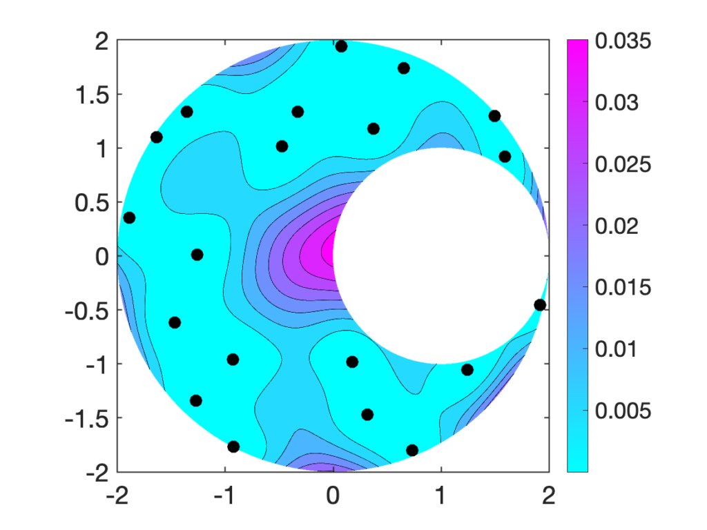
 seeks to compress a high-dimensional matrix
  or vector
  to a lower-dimensional sketched matrix
  or vector
  . The quality of a sketching matrix for a matrix
 ![\[(1-\varepsilon) \norm{x} \le \norm{Sx} \le (1+\varepsilon) \norm{x} \quad \text{for every } x \in \operatorname{col}(A).\]](https://www.ethanepperly.com/wp-content/ql-cache/quicklatex.com-06811a2d05bdccddd7b3c3079ed47729_l3.png "Rendered by QuickLaTeX.com")
 denotes the
  .
. matrix.
 (one million) and output dimension
  . For the SRTT, we use the
  .
.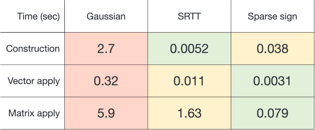
 and applying it to a matrix
  , sparse sign embeddings are 14× faster than SRTTs and 73× faster than Gaussian embeddings.
 for
for  and
and  using the MATLAB
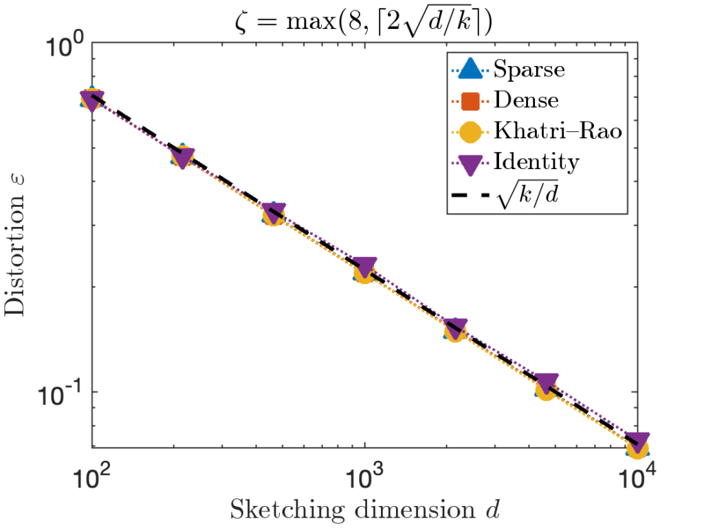
  between 100 and 10,000. We report the distortion averaged over 100 trials. The theoretically predicted value
  (equivalently,
  ) is shown as a dashed line.
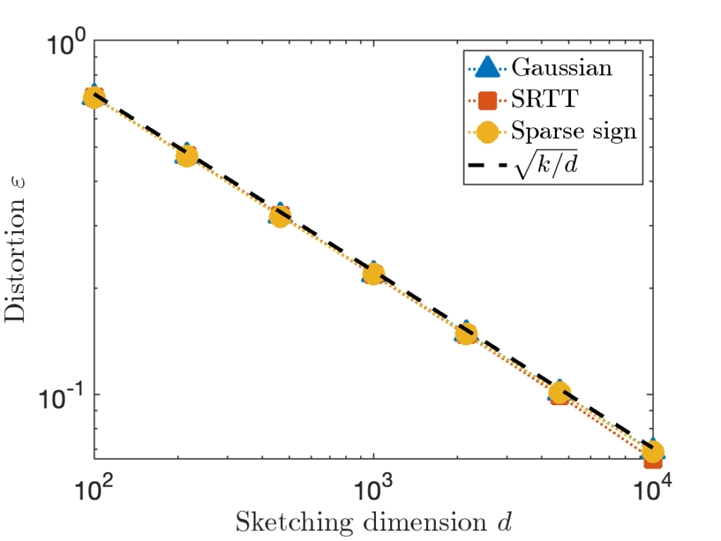
 is taken to be a matrix with independent standard Gaussian random values.
 is taken to be the
  is taken to be the
  identity matrix stacked onto a
  matrix of zeros.
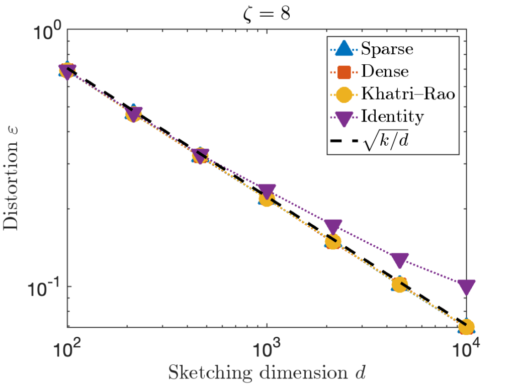
 . However, for the last test matrix “Identity”, we see the distortion begins to slightly exceed this predicted distortion for
  .
. , we can increase the value of the sparsity parameter
  . We recommend
 ![\[\zeta = \max \left( 8 , \left\lceil 2\sqrt{\frac{d}{k}} \right\rceil \right).\]](https://www.ethanepperly.com/wp-content/ql-cache/quicklatex.com-5f1ebe7695d9918399b0f97b628fcce1_l3.png "Rendered by QuickLaTeX.com")
 can be necessary to achieve the optimal distortion.
![\[S = \frac{1}{\sqrt{\zeta}} \begin{bmatrix} s_1 & \cdots & s_n \end{bmatrix}.\]](https://www.ethanepperly.com/wp-content/ql-cache/quicklatex.com-4871e53b2bb59ad11946f2d1eafc66f7_l3.png "Rendered by QuickLaTeX.com")
 is an independent and randomly generated to contain exactly
 ![\[(1-\varepsilon) \norm{x} \le \norm{Sx} \le (1+\varepsilon) \norm{x} \quad \text{for all }x \in \operatorname{col}(A).\]](https://www.ethanepperly.com/wp-content/ql-cache/quicklatex.com-41fd14292c1c85cd318dde801a75e1bd_l3.png "Rendered by QuickLaTeX.com")
![\[d = \frac{k}{\varepsilon^2} \quad \text{and} \quad \zeta = \max\left(8,\frac{2}{\varepsilon}\right).\]](https://www.ethanepperly.com/wp-content/ql-cache/quicklatex.com-ed85cec8dadffec7c7a3b4e099d6637d_l3.png "Rendered by QuickLaTeX.com")
 . The value
  has demonstrated deficiencies and should almost always be avoided (see below). The scaling
  is derived from the
 ![\[d = \mathcal{O} \left( \frac{k \log k}{\varepsilon^2} \right) \quad \text{and} \quad \zeta = \mathcal{O}\left( \frac{\log k}{\varepsilon} \right).\]](https://www.ethanepperly.com/wp-content/ql-cache/quicklatex.com-4fb6d0d60c85bc8a60d95bb0a19e63d6_l3.png "Rendered by QuickLaTeX.com")
 factor and the lack of explicit constants in the
  and can also be generated using a single line. The real challenge to generating sparse sign embeddings in MATLAB is the row indices, since each batch of
  sparse sign embedding with sparsity
  and weights
  . To apply
  and reweight them using the weights:
![\[b \in \real^n \longmapsto Sb = (w_1 b_{i_1},\ldots,w_db_{i_d}) \in \real^d.\]](https://www.ethanepperly.com/wp-content/ql-cache/quicklatex.com-712b97fc6f6efb9bf9a40dac2a652f5c_l3.png "Rendered by QuickLaTeX.com")
 for the hard “Identity” test matrix used above.
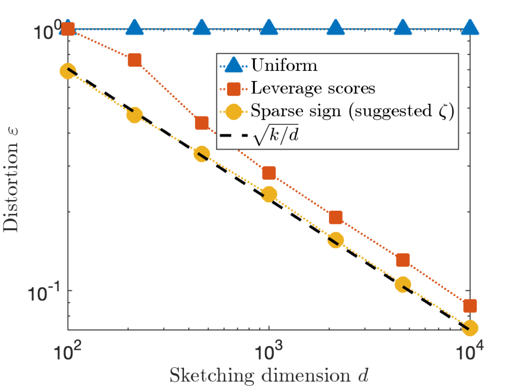
 for each row of
  cost, much higher than other types of sketches.
 , and compare the distortion of CountSketch to the sparse sign embedding with parameters
  :
: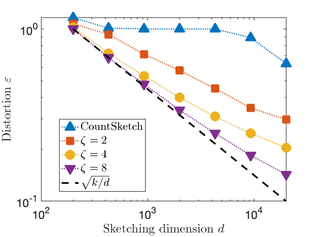
 , 20× higher than
  in order to achieve distortion
  (or perhaps
  ). This difference between
  for CountSketch and
  for other sketching matrices is a at the root of CountSketch’s woefully bad performance on some inputs.
 is an informal symbol meaning “proportional to”.
 . This is Theorem 16 in
  , where
  is a CountSketch of size
  and
and  is a Gaussian sketching matrix of size
  .
. is a CountSketch matrix with output dimension
  , then the distortion of
  with high probability.
![\[SA = \begin{bmatrix} s_1 & \cdots & s_k \end{bmatrix}\]](https://www.ethanepperly.com/wp-content/ql-cache/quicklatex.com-82c7ea0e5c52b6bd9bdb389f3d3f92d7_l3.png "Rendered by QuickLaTeX.com")
 has a single
  in a uniformly random location
  .
.
 are not all different from each other, say
  . Set
. Set  , where
  is the standard basis vector with
  but
but  . Thus, for the distortion relation
 ![\[(1-\varepsilon) \norm{x} =(1-\varepsilon)\sqrt{2} \le 0 = \norm{(SA)x}\]](https://www.ethanepperly.com/wp-content/ql-cache/quicklatex.com-b08feebb30829a0e73b02188eba6f901_l3.png "Rendered by QuickLaTeX.com")
 . Thus,
 ![\[\prob \{ \varepsilon \ge 1 \} \ge \prob \{ j_1,\ldots,j_k \text{ are not distinct} \}.\]](https://www.ethanepperly.com/wp-content/ql-cache/quicklatex.com-12fa7b716b97c7e9482f4f6327bd4728_l3.png "Rendered by QuickLaTeX.com")
 pairs of people. Each pair of people has a
  chance of sharing a birthday, so the expected number of birthdays in a room of 23 people is
  . Since are 0.69 birthdays shared on average in a room of 23 people, it is perhaps less surprising that 23 is the critical number at which the chance of two people sharing a birthday exceeds 50%.
 and
and  in CountSketch have a
  chance of being the same. There are
  pairs of indices, so the expected number of equal indices
  . Thus, we should anticipate
  is required to ensure that
 ![\[\prob \{ j_1,\ldots,j_k \text{ are not distinct} \} = 1 - \prob \{ j_1,\ldots,j_k \text{ are distinct} \}.\]](https://www.ethanepperly.com/wp-content/ql-cache/quicklatex.com-338a38501a565185b794f8ed03803c9a_l3.png "Rendered by QuickLaTeX.com")
 are all distinct, the probability
  are distinct is just the probability that
  values
 ![\[\prob\{ j_1,\ldots,j_i \text{ are distinct} \mid j_1,\ldots,j_{i-1} \text{ are distinct}\} = 1 - \frac{i-1}{d}.\]](https://www.ethanepperly.com/wp-content/ql-cache/quicklatex.com-b474f00c44e53b7c3c398d56121e1ac3_l3.png "Rendered by QuickLaTeX.com")
![\[\prob \{ j_1,\ldots,j_k \text{ are distinct} \} = \prod_{i=1}^k \left(1 - \frac{i-1}{d} \right).\]](https://www.ethanepperly.com/wp-content/ql-cache/quicklatex.com-7dd28281f8dbed8b3a1452a21e7410c8_l3.png "Rendered by QuickLaTeX.com")
 for every
  , obtaining
![\[\mathbb{P} \{ j_1,\ldots,j_k \text{ are distinct} \} \le \prod_{i=0}^{k-1} \exp\left(-\frac{i}{d}\right) = \exp \left( -\frac{1}{d}\sum_{i=0}^{k-1} i \right) = \exp\left(-\frac{k(k-1)}{2d}\right).\]](https://www.ethanepperly.com/wp-content/ql-cache/quicklatex.com-8d9d4c7d12af0fd89e53ca261c5df287_l3.png "Rendered by QuickLaTeX.com")
![\[\prob \{ \varepsilon \ge 1 \} \ge 1-\prob \{ j_1,\ldots,j_k \text{ are distinct} \\}\ge 1-\exp\left(-\frac{k(k-1)}{2d}\right).\]](https://www.ethanepperly.com/wp-content/ql-cache/quicklatex.com-144cfc73d778c4f9ed7442f5a6610e5e_l3.png "Rendered by QuickLaTeX.com")
![\[\prob\{\varepsilon \ge 1\} \ge \frac{1}{2} \quad \text{if} \quad d \le \frac{k(k-1)}{2\ln 2}.\]](https://www.ethanepperly.com/wp-content/ql-cache/quicklatex.com-e11567078a415b79b06a8e5e6f0b1600_l3.png "Rendered by QuickLaTeX.com")
 or perhaps a tall matrix
  . A sketching matrix is a
  matrix
  . When multiplied into a high-dimensional vector
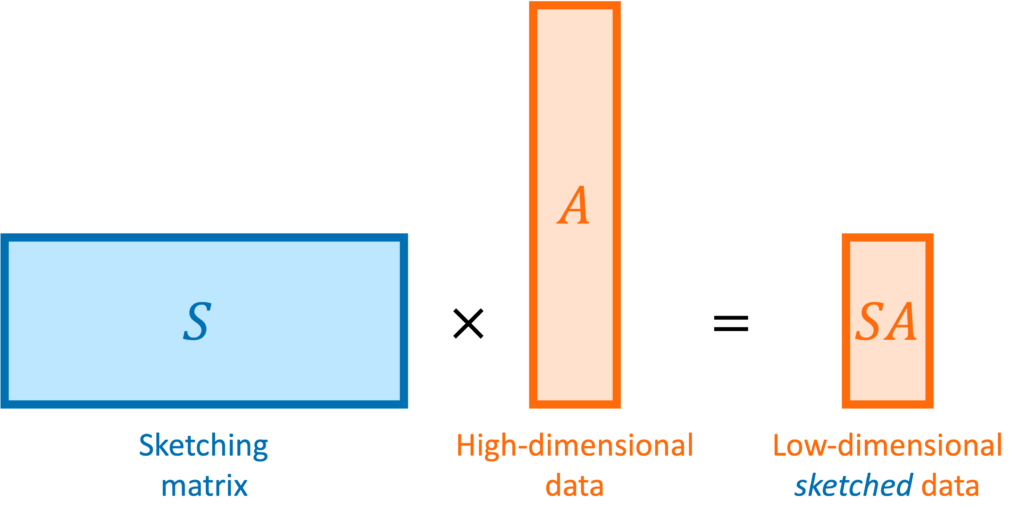
 be a collection of vectors. For
  , we require that
  :
: ![\[(1-\varepsilon) \norm{x}\le\norm{Sx}\le(1+\varepsilon)\norm{x} \]](https://www.ethanepperly.com/wp-content/ql-cache/quicklatex.com-735df49a45ff5d0bb27d478569004bdd_l3.png "Rendered by QuickLaTeX.com")
![\[\operatorname{col}(A) \coloneqq \{ Ax : x \in \real^k \}.\]](https://www.ethanepperly.com/wp-content/ql-cache/quicklatex.com-5ecde6b43df29caba14fd43682b4cc86_l3.png "Rendered by QuickLaTeX.com")
 with an output dimension of roughly
  . In particular, the sketching dimension
  elements) or dimension (
 requires roughly
  operations, rather than the
  operations we would expect to multiply a
  is
is ![\[S = \sqrt{\frac{n}{d}} \cdot R \cdot F \cdot D.\]](https://www.ethanepperly.com/wp-content/ql-cache/quicklatex.com-92095cbf9c7d55273bd572a33debe415_l3.png "Rendered by QuickLaTeX.com")
 is a diagonal matrix whose entries are each a random
  is a fast trigonometric transform such as a fast
  is a selection matrix. To generate
  , let
, let  , selected without replacement.
  for every vector
  and the
  , and
, and  operations, a significant improvement over the
  , larger than for a Gaussian sketch.
![\[S = \frac{1}{\sqrt{\zeta}} \begin{bmatrix} s_1 & s_2 & \cdots & s_n \end{bmatrix}.\]](https://www.ethanepperly.com/wp-content/ql-cache/quicklatex.com-bb5806806e2e5900d4351c08befbd82e_l3.png "Rendered by QuickLaTeX.com")
 nonzero entries. The parameter
  in practice.
 or
or  operations) to apply to a vector, depending on parameter choices (see below). With a good sparse matrix library, sparse sign embeddings are often the fastest sketching matrix by a wide margin.
 random numbers, higher than SRTTs (roughly
  numbers).
  ; the theoretically sanctioned sketching dimension (at least according to existing theory) is larger than for a Gaussian sketch. In practice, we can often get away with using
  .
. operations. Therefore, sketching offers the promise of speeding up linear algebraic computations involving
 ![\[\operatorname*{minimize}_{x\in\real^k} \norm{Ax - b}. \]](https://www.ethanepperly.com/wp-content/ql-cache/quicklatex.com-07528304ce875f54aa1173062c5ec10a_l3.png "Rendered by QuickLaTeX.com")
 . Applying
 ![\[\operatorname*{minimize}_{\hat{x}\in\real^k} \norm{(SA)\hat{x} - Sb}. \]](https://www.ethanepperly.com/wp-content/ql-cache/quicklatex.com-7110d3e9c1dd7e29793603a5bafdd201_l3.png "Rendered by QuickLaTeX.com")
 is the sketch-and-solve solution to the least-squares problem, which we can use as an approximate solution to the original least-squares problem.
 , first apply sketching to obtain
  and then apply an out-of-the-box clustering algorithms like
  denote the optimal least-squares solution and let
 ![\[\norm{A\hat{x} - b} \le \frac{1+\varepsilon}{1-\varepsilon} \norm{Ax - b}.\]](https://www.ethanepperly.com/wp-content/ql-cache/quicklatex.com-3d1d034bd8bf93f1c15e435a27a355ee_l3.png "Rendered by QuickLaTeX.com")
 , then this bound tells us that
 ![\[\norm{A\hat{x} - b} \le 2\norm{Ax_\star - b}. \]](https://www.ethanepperly.com/wp-content/ql-cache/quicklatex.com-588170743415f491f48ef2adc3d46628_l3.png "Rendered by QuickLaTeX.com")
 . For such applications, the bound (4) ensures that
  . Often, this means
  , measuring how close
  and residual norm
  ). Then, we generate a sparse sign embedding of dimension
  ). Then, we compute the sketch-and-solve solution and, as reference, a “direct” solution by
  , close to direct method’s residual norm of
  . However, the forward error of sketch-and-solve is
  nine orders of magnitude larger than the direct method’s forward error of
  .
. , to decrease the distortion by a factor of ten requires increasing the sketching dimension
  that we hope will converge at a rapid rate to the true least-squares solution,
  , then
  .
.![\[SA = QR,\]](https://www.ethanepperly.com/wp-content/ql-cache/quicklatex.com-9edf84077821e9e0cd0c772b77024799_l3.png "Rendered by QuickLaTeX.com")
![\[A^\top A \approx (SA)^\top (SA) = R^\top Q^\top Q R = R^\top R.\]](https://www.ethanepperly.com/wp-content/ql-cache/quicklatex.com-90e14ee1172525fd795980cb3ef1a647_l3.png "Rendered by QuickLaTeX.com")
 since
since  has orthonormal columns. The conclusion is that
  .
.
![\[(A^\top A)x = A^\top b. \]](https://www.ethanepperly.com/wp-content/ql-cache/quicklatex.com-3f3c5265345a169d6633a759854510da_l3.png "Rendered by QuickLaTeX.com")
 by
by  in (5) and solving. The resulting solution is
![\[x_0 = R^{-1} (R^{-\top}(A^\top b)).\]](https://www.ethanepperly.com/wp-content/ql-cache/quicklatex.com-6b63093ea5c1d9714fb0deab43fc4dc3_l3.png "Rendered by QuickLaTeX.com")
 will typically not be a good solution to the least-squares problem (2), so we need to iterate. To do so, we’ll try and solve for the error
  . To derive an equation for the error, subtract
  from both sides of the normal equations (5), yielding
 ![\[(A^\top A)(x-x_0) = A^\top (b-Ax_0).\]](https://www.ethanepperly.com/wp-content/ql-cache/quicklatex.com-4f1ee993844dbcd8e397f27ccd1deefb_l3.png "Rendered by QuickLaTeX.com")
 :
: ![\[x\approx x_1 \coloneqq x_0 + R^{-\top}(R^{-1}(A^\top(b-Ax_0))).\]](https://www.ethanepperly.com/wp-content/ql-cache/quicklatex.com-0496d7e3c8bc117e658c57fc167081be_l3.png "Rendered by QuickLaTeX.com")
 , approximate
  , and obtain a new approximate solution
  . Continuing this process, we obtain an iteration
![\[x_{i+1} = x_i + R^{-\top}(R^{-1}(A^\top(b-Ax_i))).\]](https://www.ethanepperly.com/wp-content/ql-cache/quicklatex.com-f8db238fc978e6a8fc968fc5e387ec27_l3.png "Rendered by QuickLaTeX.com")
 at every iteration. Later,
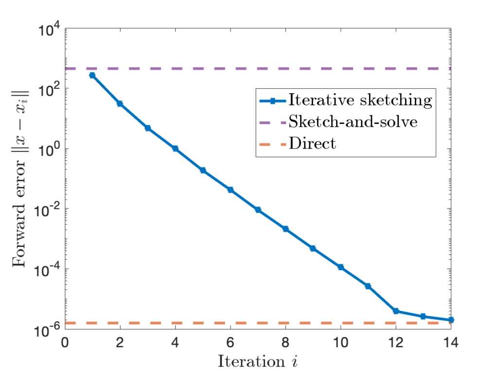
 to
to  , the accuracy of the iterative sketching solution
  can be quite high.
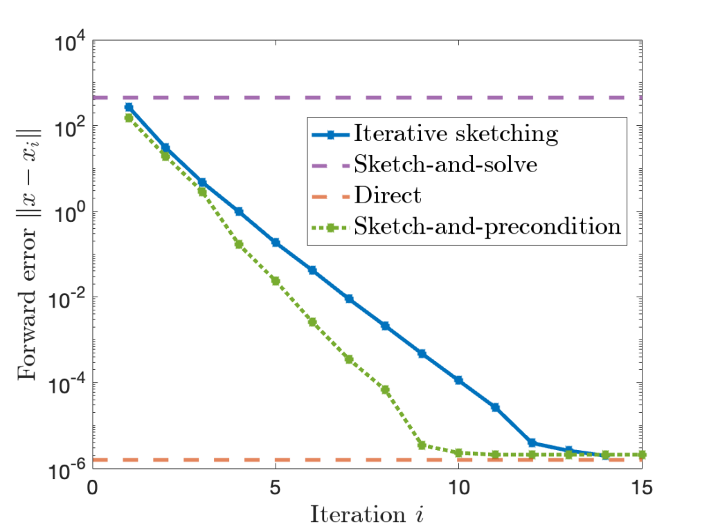
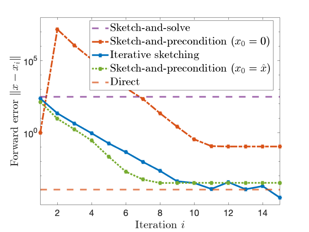
 is comparable to accuracy of a standard
  , sketch-and-precondition is not forward stable. The maximum achievable accuracy was worse than standard solvers by orders of magnitude! Maybe sketching doesn’t work after all?
 for sketch-and-precondition, then sketch-and-precondition appears to be forward stable in practice. No theoretical analysis supporting this finding is known at present.
 and residual
  .
.
 a
a  and
and  are defined. Then
 ![f(\mathbb{E}X) \le \mathbb{E} [f(X)]](https://www.ethanepperly.com/wp-content/ql-cache/quicklatex.com-be01f50345229c7ba054de409859eec8_l3.png "Rendered by QuickLaTeX.com") .
. , there exists a slope
  for all
  and
and  and take expectations to conclude that
![\[\mathbb{E}[m(X - \mathbb{E}X) + f(\mathbb{E}X)] = f(\mathbb{E}X) \le \mathbb{E} [f(X)].\]](https://www.ethanepperly.com/wp-content/ql-cache/quicklatex.com-c162fcb6103e44c65d3c6e1d003135d0_l3.png "Rendered by QuickLaTeX.com")
 for two numbers
  and
and  . This may hard to do directly. With the interpolation method, I first construct a family of numbers
  ,
,  , such that
  and
and  and show that
  is (weakly) increasing in
  . This is typically accomplished by showing the derivative is nonnegative:
![\[\frac{d}{dt} A_t \ge 0.\]](https://www.ethanepperly.com/wp-content/ql-cache/quicklatex.com-7d87bd05d1a5b326f575b2b72f27cc74_l3.png "Rendered by QuickLaTeX.com")
 for some
  for any Gaussian random variable
  .
.![\[f(0) \le \mathbb{E} [f(X)].\]](https://www.ethanepperly.com/wp-content/ql-cache/quicklatex.com-8e5dd3a04978ca82dd4d50fd41f8ca43_l3.png "Rendered by QuickLaTeX.com")
![\[A_t = \mathbb{E} [ f(X_t) ],\]](https://www.ethanepperly.com/wp-content/ql-cache/quicklatex.com-8f12251961aff234ee138a29978a264b_l3.png "Rendered by QuickLaTeX.com")
 starts with no randomness and
  is our standard Gaussian. To interpolate between these extremes, we increase the variance linearly from
  to
to ![\[A_t = \mathbb{E} [ f(X_t)] \quad \text{where $X_t\sim\mathcal{N}(0,t)$}.\]](https://www.ethanepperly.com/wp-content/ql-cache/quicklatex.com-88cc0a1a3f5c52e8349fd6c4ca28ad7c_l3.png "Rendered by QuickLaTeX.com")
 denotes a Gaussian random variable with zero mean and variance
  denote a small parameter which we will later send to zero. For us, the key fact will be that a
  can be realized as a sum of independent
  and
and  random variables. Therefore, we write
![\[X_{t+\delta} = X_t + \Delta \quad \text{where $\Delta \sim \mathcal{N}(0,\delta)$ is independent of $X_t$.}\]](https://www.ethanepperly.com/wp-content/ql-cache/quicklatex.com-eaaa1bd888269b9ad51b88afb5fc3d08_l3.png "Rendered by QuickLaTeX.com")
 by using Taylor’s formula
![\[f(X_t+\Delta) = f(X_t) + f'(X_t)\Delta + \frac{1}{2} f''(X_t) \Delta^2 + \frac{1}{6} f'''(\xi) \Delta^3, \]](https://www.ethanepperly.com/wp-content/ql-cache/quicklatex.com-38d38dde93cc24a3101649064d5af389_l3.png "Rendered by QuickLaTeX.com")
 lies between
  and
and  . Now, take expectations,
 ![\[\mathbb{E}[ f(X_t+\Delta)]=\mathbb{E}[f(X_t)] + \mathbb{E}[f'(X_t)\Delta] + \frac{1}{2} \mathbb{E}[f''(X_t)] \mathbb{E}[\Delta^2] + \underbrace{\frac{1}{6} \mathbb{E}[f'''(\xi) \Delta^3]}_{:=\mathrm{Rem}(\delta)}.\]](https://www.ethanepperly.com/wp-content/ql-cache/quicklatex.com-ccacfa2622a31446e66624a9a8458dc4_l3.png "Rendered by QuickLaTeX.com")
 has mean zero and variance
  so this gives
![\[\mathbb{E} [f(X_t+\Delta)]=\mathbb{E}[f(X_t)] + \delta \frac{1}{2} \mathbb{E}[f''(X_t)] + \mathrm{Rem}(\delta).\]](https://www.ethanepperly.com/wp-content/ql-cache/quicklatex.com-d021f960b2367c41cf18dc25661045c6_l3.png "Rendered by QuickLaTeX.com")
 vanishes as
  . Thus, we can rearrange this expression to compute the derivative:
![\[\frac{d}{dt} A_t = \lim_{\delta \downarrow 0} \frac{\mathbb{E} f(X_t+\Delta)-\mathbb{E}[f(X_t)]}{\delta} = \lim_{\delta \downarrow 0} \frac{1}{2} \mathbb{E}[f''(X_t)] + \frac{\mathrm{Rem}(\delta)}{\delta} = \frac{1}{2} \mathbb{E}[f''(X_t)].\]](https://www.ethanepperly.com/wp-content/ql-cache/quicklatex.com-3275fd914e25d0f6985eb4d1ca419fb7_l3.png "Rendered by QuickLaTeX.com")
 for every
 ![\[\frac{d}{dt} A_t \ge 0 \quad \text{for all } t\in [0,1].\]](https://www.ethanepperly.com/wp-content/ql-cache/quicklatex.com-258c784d449d2b53c0a462ff38f3cdd8_l3.png "Rendered by QuickLaTeX.com")
![\[\mathbb{E} f(X) = f(0) + \frac{1}{2} \int_0^1 \mathbb{E} [f''(X_t)] \, dt.\]](https://www.ethanepperly.com/wp-content/ql-cache/quicklatex.com-50be5d67c30ff436025f45185c2fae22_l3.png "Rendered by QuickLaTeX.com")

![\[f''(x) \le \beta \quad \text{for every } x \in \real,\]](https://www.ethanepperly.com/wp-content/ql-cache/quicklatex.com-206d02bd0b654ab4c42cf33921d5383d_l3.png "Rendered by QuickLaTeX.com")
![\[f(0) \le \mathbb{E} f(X) \le f(0) + \frac{1}{2}\beta.\]](https://www.ethanepperly.com/wp-content/ql-cache/quicklatex.com-8561680db386f740b927a84c7cb9fe0d_l3.png "Rendered by QuickLaTeX.com")
 . Let’s do this. As an exercise, you can verify that our technical regularity condition implies
  . Thus, by Hölder’s inequality and setting
  ), we obtain
![\[\frac{|\mathrm{Rem}(\delta)|}{\delta} = \frac{|\mathbb{E}[f'''(\xi) \Delta^3]|}{6\delta} \le \frac{(|\mathbb{E} |f'''(\xi)|^p)^{1/p}| (\mathbb{E} |\Delta|^{3q})^{1/q}}{6\delta}.\]](https://www.ethanepperly.com/wp-content/ql-cache/quicklatex.com-e1078e0f2d2c17b77bd87a38665c03e4_l3.png "Rendered by QuickLaTeX.com")
 where
where  is a function of
  as
as  .
. , defined for each
  . Rather than treating these quantities as independent, we can think of them as a collective, comprising a random function
  known as a
![\[df = f'(x) \, dx\]](https://www.ethanepperly.com/wp-content/ql-cache/quicklatex.com-a32870f7f5981a412b96de2591534280_l3.png "Rendered by QuickLaTeX.com")
 of a Brownian motion, the analog is
 ![\[df = f'(X_t) \, dX_t + \frac{1}{2} f''(X_t) \, dt.\]](https://www.ethanepperly.com/wp-content/ql-cache/quicklatex.com-e2eadd9f0624f41b562d90fe0568ef69_l3.png "Rendered by QuickLaTeX.com")
 over a time interval
  ,
,  is a random variable with mean
 ![\[f(\mathbb{E}Y) \le \mathbb{E}[f(Y)].\]](https://www.ethanepperly.com/wp-content/ql-cache/quicklatex.com-97693077e012820448760d2e7ad31d58_l3.png "Rendered by QuickLaTeX.com")
 and
and  denote the cumulative distribution functions of
 ![\[g(X) := \inf \{ \alpha \in \real : F_Y(\alpha) \ge F_X(X) \}\]](https://www.ethanepperly.com/wp-content/ql-cache/quicklatex.com-2c40cdc3f3bcf589f930aeb87340491b_l3.png "Rendered by QuickLaTeX.com")
 and
and ![\[A_t \stackrel{?}{=} \mathbb{E} [f(g(X_t))].\]](https://www.ethanepperly.com/wp-content/ql-cache/quicklatex.com-0de3d1811026212f153ea79469649149_l3.png "Rendered by QuickLaTeX.com")
![A_0 = \mathbb{E}[f(g(0))]](https://www.ethanepperly.com/wp-content/ql-cache/quicklatex.com-e6ac6421e3fc94f2087614f41336491a_l3.png "Rendered by QuickLaTeX.com") does not even equal to
does not even equal to ![\mathbb{E} [f(Y)]](https://www.ethanepperly.com/wp-content/ql-cache/quicklatex.com-06983640d9e119e9aa44cdd209c540c7_l3.png "Rendered by QuickLaTeX.com") ! Instead, we must define
! Instead, we must define![\[A_t = \mathbb{E} [f(\mathbb{E}[g(X_1) \mid X_t])].\]](https://www.ethanepperly.com/wp-content/ql-cache/quicklatex.com-19560c3c89aa3987101e6650af24a0a7_l3.png "Rendered by QuickLaTeX.com")
 conditional on the Brownian motion
 ![\[\frac{d}{dt} A_t \ge 0 \quad \text{for all }t\in [0,1].\]](https://www.ethanepperly.com/wp-content/ql-cache/quicklatex.com-253003b644ae67d253cdfd74378c71a9_l3.png "Rendered by QuickLaTeX.com")
 are “somewhat dependent”, for which functions does the multivariate Jensen’s inequality
  )
) ![\[f(\mathbb{E} Y_1,\ldots,\mathbb{E}Y_n) \le \mathbb{E} [f(Y_1,\ldots,Y_n)] \]](https://www.ethanepperly.com/wp-content/ql-cache/quicklatex.com-2467fe840ba04173b1a3adc7c38a945c_l3.png "Rendered by QuickLaTeX.com")
![\[\text{($\star$) holds if $f$ is convex in each coordinate, separately.}\]](https://www.ethanepperly.com/wp-content/ql-cache/quicklatex.com-521f389e0e1a83728c2544ecb889a047_l3.png "Rendered by QuickLaTeX.com")
 of Gaussian random variables
  . We will use the covariance matrix
  of the Gaussian random variables
 ![\[f(\mathbb{E}g_1(X_1),\ldots,\mathbb{E}g_n(X_n)) \le \mathbb{E} [f(g(X_1),\ldots,g(X_n))]\]](https://www.ethanepperly.com/wp-content/ql-cache/quicklatex.com-055c60480c4de2b28348bb1da12763ea_l3.png "Rendered by QuickLaTeX.com")
 if and only if
 ![\[\Sigma \circ \nabla^2 f(x) \text{ is positive semidefinite} \quad \text{for all $x \in \real^n$}.\]](https://www.ethanepperly.com/wp-content/ql-cache/quicklatex.com-48ca7d18e3bbcee337d072bd27efe791_l3.png "Rendered by QuickLaTeX.com")
 is the
  denotes the
  are equal (and variance one),
  for all
 ![\[\Sigma \circ \nabla^2 f(x) = \mathrm{diag} \left( \frac{\partial^2 f}{\partial x_i^2} : i=1,\ldots,n \right).\]](https://www.ethanepperly.com/wp-content/ql-cache/quicklatex.com-ef80f7d5a452131378d194e3560717b0_l3.png "Rendered by QuickLaTeX.com")
 : this is precisely the condition for
  , estimate its trace
  .
.![\[\hat{\tr} = \frac{1}{m} \sum_{i=1}^m \omega_i^* A \omega_i. \]](https://www.ethanepperly.com/wp-content/ql-cache/quicklatex.com-a287886ee24c9ab99dfe35b6cdae83cf_l3.png "Rendered by QuickLaTeX.com")
 are random vectors, usually chosen to be
  denotes the
  .
.![\[\mathbb{E} [\omega_i\omega_i^*] = I, \]](https://www.ethanepperly.com/wp-content/ql-cache/quicklatex.com-74bb76367ad1408bd538d049774cf990_l3.png "Rendered by QuickLaTeX.com")
![\[\mathbb{E} [\hat{\tr}] = \tr A.\]](https://www.ethanepperly.com/wp-content/ql-cache/quicklatex.com-f6407c7a741003cc20780e72d050cb56_l3.png "Rendered by QuickLaTeX.com")
![\[\mathbb{E} [\hat{\tr}] = \mathbb{E} \left[ \frac{1}{m} \sum_{i=1}^m \omega_i^*A\omega_i \right] = \frac{1}{m} \sum_{i=1}^m \mathbb{E} \left[ \omega_i^* A \omega_i\right]. \]](https://www.ethanepperly.com/wp-content/ql-cache/quicklatex.com-52eebd003a597cac5b2c69f7b6e537e8_l3.png "Rendered by QuickLaTeX.com")
![\mathbb{E} [\hat{\tr}] = \tr A](https://www.ethanepperly.com/wp-content/ql-cache/quicklatex.com-96f71a1b054ffed9e316cf9cb7a16c5c_l3.png "Rendered by QuickLaTeX.com") , it is sufficient to prove that
, it is sufficient to prove that ![\mathbb{E} \left[\omega_i^*A\omega_i\right] = \tr A](https://www.ethanepperly.com/wp-content/ql-cache/quicklatex.com-120169dca277175c51f09b6f320cf5fa_l3.png "Rendered by QuickLaTeX.com") for each
for each  matrix, then a number equals its trace,
  . The second trick is the
  matrix
  and a
and a  matrix
  , we have
  . The cyclic property
 ![\[\tr[BCD] = \tr[(BC)D] = \tr[D(BC)] = \tr[DBC].\]](https://www.ethanepperly.com/wp-content/ql-cache/quicklatex.com-cc1cd4920a2431e93b5453b5373999e3_l3.png "Rendered by QuickLaTeX.com")
![\[\tr [BCD] \ne \tr[CBD] \quad \text{in general}.\]](https://www.ethanepperly.com/wp-content/ql-cache/quicklatex.com-f563660fc58383a37ae7bedea16b2b9c_l3.png "Rendered by QuickLaTeX.com")
 as beads on a closed loop of string. One can move the last bead
 ![\tr [BCD] = \tr[DBC]](https://www.ethanepperly.com/wp-content/ql-cache/quicklatex.com-7656627b133add21ab8765532def07d6_l3.png "Rendered by QuickLaTeX.com") , but not interchange two beads,
, but not interchange two beads, ![\tr[BCD] \ne \tr[CBD]](https://www.ethanepperly.com/wp-content/ql-cache/quicklatex.com-0f43e4f72510a69b596f7b9f7504dd58_l3.png "Rendered by QuickLaTeX.com") .
.![\[\mathbb{E} \left[\omega_i^*A\omega_i\right] = \mathbb{E} \tr \left[\omega_i^*A\omega_i\right] = \mathbb{E} \tr \left[A\omega_i\omega_i^*\right].\]](https://www.ethanepperly.com/wp-content/ql-cache/quicklatex.com-b1bb373766e64179bc0635f058a07f3f_l3.png "Rendered by QuickLaTeX.com")
![\[\mathbb{E} \left[\omega_i^*A\omega_i\right] = \mathbb{E} \tr \left[A\omega_i\omega_i^*\right] = \tr(A \mathbb{E}[\omega_i\omega_i^*] ).\]](https://www.ethanepperly.com/wp-content/ql-cache/quicklatex.com-1d10f835c99efab005f0ad12cdb5647b_l3.png "Rendered by QuickLaTeX.com")
![\[\mathbb{E} \left[\omega_i^*A\omega_i\right] = \tr(A \mathbb{E}[\omega_i\omega_i^*] ) = \tr(A\cdot I) = \tr A.\]](https://www.ethanepperly.com/wp-content/ql-cache/quicklatex.com-b51781498146df3547c1503e451ad682_l3.png "Rendered by QuickLaTeX.com")
 ‘s are isotropic (3) and now assume that
 ![\[\Var(\hat{\tr}) = \frac{1}{m^2} \sum_{i=1}^m \Var(\omega_i^*A\omega_i).\]](https://www.ethanepperly.com/wp-content/ql-cache/quicklatex.com-d9398dc43178ba9bb72aead0214e77c8_l3.png "Rendered by QuickLaTeX.com")
 , we then get
![\[\Var(\hat{\tr}) = \frac{1}{m} \Var(\omega^*A\omega).\]](https://www.ethanepperly.com/wp-content/ql-cache/quicklatex.com-4501a18842234362f8f99d523c7c723e_l3.png "Rendered by QuickLaTeX.com")
 , which is characteristic of
 ![\[\left| \hat{\tr} - \tr A \right| \lessapprox \frac{\mathrm{const}}{\sqrt{m}}.\]](https://www.ethanepperly.com/wp-content/ql-cache/quicklatex.com-c735791b8fe88d627bc2ebad8137fb1e_l3.png "Rendered by QuickLaTeX.com")
 , I must do
  the work!
 and (root-mean-square) error at rates
 ![\[\Var(\hat{\tr}_{\text{H++ or X}}) \le \frac{\mathrm{const}}{m^2},\quad \left| \hat{\tr}_{\text{H++ or X}} - \tr A \right| \lessapprox \frac{\mathrm{const}}{m}.\]](https://www.ethanepperly.com/wp-content/ql-cache/quicklatex.com-87438d87094d3df389400b5f7abee24a_l3.png "Rendered by QuickLaTeX.com")
 that makes the variance of the single–sample estimate
  as low as possible. In this section, we will provide several explicit formulas for the variance of the Girard–Hutchinson estimator. Derivations of these formulas will appear at the end of this post. These variance formulas help illuminate the benefits and drawbacks of different test vector distributions.
 we use
  and
and  to denote the real and imaginary parts. The variance of a random complex number
 ![\[\Var(z) := \mathbb{E} |z - \mathbb{E} z|^2 = \Var(\Re z) + \Var(\Im z).\]](https://www.ethanepperly.com/wp-content/ql-cache/quicklatex.com-8f636667a7dbbb3217896a962de1d28c_l3.png "Rendered by QuickLaTeX.com")
![\[\left\|A\right\|_{\rm F}^2 = \sum_{i,j} |A_{ij}|^2.\]](https://www.ethanepperly.com/wp-content/ql-cache/quicklatex.com-e132e4b9029c41dbfb99cd0e588d8d70_l3.png "Rendered by QuickLaTeX.com")
 , we have
![\[\left\|A\right\|_{\rm F}^2 = \sum_{i=1}^n \lambda_i^2. \]](https://www.ethanepperly.com/wp-content/ql-cache/quicklatex.com-06b272e602552353c020f6399347c748_l3.png "Rendered by QuickLaTeX.com")
 denotes the
  denotes the
  rather than the conjugate transpose
  is a number, it is equal to its own transpose:
![\[\omega^\top A \omega = (\omega^\top A \omega)^\top = \omega^\top A^\top \omega.\]](https://www.ethanepperly.com/wp-content/ql-cache/quicklatex.com-3d543dc0d4d64d3c28f0f291cd9c8e83_l3.png "Rendered by QuickLaTeX.com")
![\[\omega^\top A\omega = \frac{\omega^\top A \omega + \omega^\top A^\top \omega}{2} = \omega^\top \left( \frac{A + A^\top}{2} \right)\omega.\]](https://www.ethanepperly.com/wp-content/ql-cache/quicklatex.com-f1bbe4f0c983f73e2461b593b752f54a_l3.png "Rendered by QuickLaTeX.com")
 .
. .
.![\[\Var(\omega^\top A\omega) = 2 \left\|A\right\|_{\rm F}^2.\]](https://www.ethanepperly.com/wp-content/ql-cache/quicklatex.com-091cf638fab943be5fd224acdb42668f_l3.png "Rendered by QuickLaTeX.com")
![\[\Var(\omega^\top A \omega) = 2\sum_{i\ne j} |A_{ij}|^2.\]](https://www.ethanepperly.com/wp-content/ql-cache/quicklatex.com-74621dad79cb3f06a8b70c661df4e01d_l3.png "Rendered by QuickLaTeX.com")
 are uniformly distributed on the real sphere of radius
  .
. ![\[\Var(\omega^\top A\omega) = \frac{2n}{n+2} \left( \left\|A\right\|_{\rm F}^2 - \frac{1}{n} |\tr A|^2 \right).\]](https://www.ethanepperly.com/wp-content/ql-cache/quicklatex.com-1e419b8da9b953a0b8b914df9e89f8c6_l3.png "Rendered by QuickLaTeX.com")
![\[A = A^{\rm H} + i A^{\rm SH}\]](https://www.ethanepperly.com/wp-content/ql-cache/quicklatex.com-d61da43cd6497ceefd2306aabb52ee67_l3.png "Rendered by QuickLaTeX.com")
![\[A^{\rm H} = \frac{A+A^*}{2} ,\quad A^{\rm SH} = \frac{A - A^*}{2i}\]](https://www.ethanepperly.com/wp-content/ql-cache/quicklatex.com-dc287a49a59dca9421fdd2bef6be5334_l3.png "Rendered by QuickLaTeX.com")
 is skew-Hermitian). Since
  and
and  are both Hermitian, we have
![\[\Re(\omega^* A\omega) = \omega^* A^{\rm H} \omega, \quad \Im (\omega^* A \omega) = \omega^* A^{\rm SH} \omega.\]](https://www.ethanepperly.com/wp-content/ql-cache/quicklatex.com-6809a35cd06d92218ce8d597847f74bd_l3.png "Rendered by QuickLaTeX.com")
 can be broken into Hermitian and skew-Hermitian parts:
![\[\Var(\omega^* A\omega) = \Var(\omega^* A^{\rm H}\omega) + \Var(\omega^* A^{\rm SH}\omega).\]](https://www.ethanepperly.com/wp-content/ql-cache/quicklatex.com-e4658c38df479c5805dabd94b64cc0b3_l3.png "Rendered by QuickLaTeX.com")
 .
. for
for  standard normal random variables.
 ![\[\Var(\omega^* A\omega) = \left\|A\right\|_{\rm F}^2.\]](https://www.ethanepperly.com/wp-content/ql-cache/quicklatex.com-1beb66e032d83431dac6f8e0d6655eec_l3.png "Rendered by QuickLaTeX.com")
 .
. ![\[\Var(\omega^* A \omega) = \sum_{i\ne j} |A_{ij}|^2.\]](https://www.ethanepperly.com/wp-content/ql-cache/quicklatex.com-1cb0e8df66c34056cd350752070af17a_l3.png "Rendered by QuickLaTeX.com")
 .
. ![\[\Var(\omega^* A\omega) = \frac{n}{n+1} \left( \left\|A\right\|_{\rm F}^2 - \frac{1}{n} |\tr A|^2 \right).\]](https://www.ethanepperly.com/wp-content/ql-cache/quicklatex.com-aacfa2afb45905f6abe0697c769cd1b7_l3.png "Rendered by QuickLaTeX.com")
 are isotropic (2), independent from each other, and have independent entries, then for any fixed real symmetric matrix
  .
. -valued and an
  -valued test vectors on unified footing, let
  denote either
  ) or a complex Hermitian matrix (if
  ). Let a
  of
of ![\[\text{If $A \in \mathscr{A}$ and $U$ is $\field$-unitary, then $U^*AU \in \mathscr{A}$.}\]](https://www.ethanepperly.com/wp-content/ql-cache/quicklatex.com-18b4216d44b2364ea39ed4a078a067af_l3.png "Rendered by QuickLaTeX.com")
 is minimized by choosing
  .
. , the set of all
  , where
  is a diagonal matrix reporting
  has the same distribution as
  . Therefore,
![\[\Var(\omega^\top A \omega) = \Var(\omega^\top \Lambda \omega) = \Var \left( \sum_{i=1}^n \lambda_i \omega_i^2 \right) = \sum_{i=1}^n \lambda_i^2 \Var(\omega_i^2) = 2\sum_{i=1}^n \lambda_i^2 = 2\left\|A\right\|_{\rm F}^2.\]](https://www.ethanepperly.com/wp-content/ql-cache/quicklatex.com-a7416823720bac922fae7cc685892a49_l3.png "Rendered by QuickLaTeX.com")
 . Thus,
![\[\Var(\omega^\top A \omega) = \Var(\omega^\top \mathfrak{R}(A) \omega) + \Var(\omega^\top \mathfrak{I}(A) \omega) = 2\left\|\mathfrak{R}(A)\right\|_{\rm F}^2 + 2\left\|\mathfrak{I}(A)\right\|_{\rm F}^2 = 2\left\|A\right\|_{\rm F}^2.\]](https://www.ethanepperly.com/wp-content/ql-cache/quicklatex.com-527980eb3510f2c015106e6945126d41_l3.png "Rendered by QuickLaTeX.com")
![\[\omega^\top A \omega - \mathbb{E}[\omega^\top A \omega] = \sum_{i,j=1}^n A_{ij} \omega_i\omega_j - \sum_{i=1}^n A_{ii} = \sum_{i\ne j} A_{ij} \omega_i\omega_j + \sum_{i=1}^n A_{ii}(\omega_i^2-1).\]](https://www.ethanepperly.com/wp-content/ql-cache/quicklatex.com-4489cc9cb97ee7a0896bc61193d79910_l3.png "Rendered by QuickLaTeX.com")
 for every
  can be replaced by two times the sum over
  :
:![\[\omega^\top A \omega - \mathbb{E}[\omega^\top A \omega] = 2\sum_{i< j} A_{ij} \omega_i\omega_j.\]](https://www.ethanepperly.com/wp-content/ql-cache/quicklatex.com-afc5f6bb40cd00b7897f25d73751f4ca_l3.png "Rendered by QuickLaTeX.com")
 are
are ![\[\Var(a_1 X_1+\cdots+a_kX_k) = |a_1|^2 \Var(X_1) + \cdots + |a_k|^2 \Var(X_k)\]](https://www.ethanepperly.com/wp-content/ql-cache/quicklatex.com-b6fd81d15f564f514f79ab4c33d133d8_l3.png "Rendered by QuickLaTeX.com")
 and numbers
  . Ergo,
![\begin{align*}\Var(\omega^\top A\omega) &= \Var(\omega^\top A \omega - \mathbb{E}[\omega^\top A \omega]) \\&= \Var\left(\sum_{i< j} 2A_{ij} \omega_i\omega_j\right) \\&= \sum_{i<j} 4 |A_{ij}|^2 \Var(\omega_i\omega_j) \\&= \sum_{i<j} 4 |A_{ij}|^2 \\&= 2 \sum_{i\ne j} |A_{ij}|^2.\end{align*}](https://www.ethanepperly.com/wp-content/ql-cache/quicklatex.com-bbb33f378fabd391c28d938420d3a32b_l3.png "Rendered by QuickLaTeX.com")
 is a uniform random sign, which has variance
  camels, the second son took
  camels, the third son
  camels and the wise man took his own camel and went away.
 is easy. Fortunately, we already know such a distribution, the Gaussian distribution, for which we already calculated
  .
.![\[g = \sqrt{\frac{a}{n}} \omega,\]](https://www.ethanepperly.com/wp-content/ql-cache/quicklatex.com-a93345cf94749f98e715e42bc796501c_l3.png "Rendered by QuickLaTeX.com")
 is the squared length of the Gaussian vector
 using the
 ![\[\Var(g^\top A g) = \mathbb{E}[\Var(g^\top A g \mid a)] + \Var(\mathbb{E}[g^\top A g \mid a]).\]](https://www.ethanepperly.com/wp-content/ql-cache/quicklatex.com-e4e5ed235fbf5b2e026bcc58bd23becc_l3.png "Rendered by QuickLaTeX.com")
 and
and ![\mathbb{E}[ \cdot \mid a]](https://www.ethanepperly.com/wp-content/ql-cache/quicklatex.com-6035d77442675ac2f790cfb5417e1072_l3.png "Rendered by QuickLaTeX.com") denote the
denote the  and treating
 ![\begin{align*}\Var(g^\top A g) &= \mathbb{E}[\Var(a/n \cdot \omega^\top A \omega \mid a)] + \Var(\mathbb{E}[a/n \cdot \omega^\top A \omega \mid a]) \\&=\mathbb{E}[(a/n)^2\Var(\omega^\top A \omega)] + \Var(a/n \cdot \mathbb{E}[\omega^\top A \omega]) \\&= \frac{1}{n^2} \mathbb{E}[a^2] \cdot \Var(\omega^\top A \omega) + \frac{1}{n^2} \Var(a) |\mathbb{E} [\omega^\top A \omega]|^2.\end{align*}](https://www.ethanepperly.com/wp-content/ql-cache/quicklatex.com-be052caddf1d08941925fa0283784635_l3.png "Rendered by QuickLaTeX.com")
![\mathbb{E}[a^2]](https://www.ethanepperly.com/wp-content/ql-cache/quicklatex.com-53042ba72cdd3991b14b5d4508da6564_l3.png "Rendered by QuickLaTeX.com") and
and  are known quantities that
 ![\[\mathbb{E}[a^2] = n(n+2), \quad \Var(a) = 2n.\]](https://www.ethanepperly.com/wp-content/ql-cache/quicklatex.com-59ecda0ea21d92e43e3182d5cc5a7217_l3.png "Rendered by QuickLaTeX.com")
![\mathbb{E} [\omega^\top A \omega] = \tr A](https://www.ethanepperly.com/wp-content/ql-cache/quicklatex.com-293908b9583df45d93349435d76b981a_l3.png "Rendered by QuickLaTeX.com") . Plugging these all in, we get
. Plugging these all in, we get![\[2\left\|A\right\|_{\rm F}^2 = \frac{n+2}{n} \Var(\omega^\top A\omega) + \frac{2}{n} |\tr A|^2.\]](https://www.ethanepperly.com/wp-content/ql-cache/quicklatex.com-1c9b70fd4e5bc6ca4006114830d45619_l3.png "Rendered by QuickLaTeX.com")
![\[\Var(\omega^\top A\omega) = \frac{2n}{n+2} \left( \left\|A\right\|_{\rm F}^2 - \frac{1}{n}|\tr A|^2\right).\]](https://www.ethanepperly.com/wp-content/ql-cache/quicklatex.com-7ab53e5895f9a1f474f5bf99fbec5662_l3.png "Rendered by QuickLaTeX.com")
![\[\Var(\omega^*A \omega) = \Var \left( \sum_{i=1}^n \lambda_i |\omega_i|^2 \right) = \sum_{i=1}^n \Var(|\omega_i|^2) \lambda_i^2 = \sum_{i=1}^n \lambda_i^2 = \left\|A\right\|_{\rm F}^2.\]](https://www.ethanepperly.com/wp-content/ql-cache/quicklatex.com-68f4685a4cd845b98fc1a8fd1494e00a_l3.png "Rendered by QuickLaTeX.com")
 is a
is a  ) reveals that
![\[\Var\left( \omega^* A \omega \right) = \Var \left( \sum_{i<j} 2 \Re(A_{ij} \overline{\omega_i} \omega_j) \right).\]](https://www.ethanepperly.com/wp-content/ql-cache/quicklatex.com-b0e61723c22b056d1aca51694c407e6d_l3.png "Rendered by QuickLaTeX.com")
 are
are ![\[\Var\left( \omega^* A \omega \right) = \Var \left( \sum_{i<j} 2 \Re(A_{ij} \overline{\omega_i} \omega_j) \right) = 4\sum_{i<j} \Var \left( \Re(A_{ij} \overline{\omega_i} \omega_j) \right).\]](https://www.ethanepperly.com/wp-content/ql-cache/quicklatex.com-f2d77eb554a1e1ffbe4370efd8c704fb_l3.png "Rendered by QuickLaTeX.com")
 is uniformly distributed on the complex unit circle, we can assume without loss of generality that
  . Thus, letting
  be uniform on the complex unit circle,
![\[\Var\left( \omega^* A \omega \right) = 4\sum_{i<j} \Var \left( |A_{ij}|\Re(\phi)) \right) = 4\Var\left( \Re(\phi) \right)\sum_{i<j}|A_{ij}|^2.\]](https://www.ethanepperly.com/wp-content/ql-cache/quicklatex.com-76d2ce84714c4549a86686259bd96847_l3.png "Rendered by QuickLaTeX.com")
![\[1 = \Var(\phi) = \Var(\Re \phi) + \Var(\Im \phi) = 2 \Var(\Re \phi)\]](https://www.ethanepperly.com/wp-content/ql-cache/quicklatex.com-f83462ae4de80311482849de445edd5a_l3.png "Rendered by QuickLaTeX.com")
 . Thus
![\[\Var\left( \omega^* A \omega \right) = 2 \sum_{i<j}|A_{ij}|^2 = \sum_{i\ne j} |A_{ij}|^2.\]](https://www.ethanepperly.com/wp-content/ql-cache/quicklatex.com-436eeb79ad0eddde0752f1a398397ad5_l3.png "Rendered by QuickLaTeX.com")
 and
and  denote the real and imaginary parts of a vector or matrix, taken entrywise. The key insight is that if
 ![\[\mathscr{R}(\omega) := \twobyone{\mathfrak{R}(\omega)}{\mathfrak{I}(\omega)}\in\real^{2n} \quad \text{is a uniform random vector on the real sphere of radius $\sqrt{n}$}.\]](https://www.ethanepperly.com/wp-content/ql-cache/quicklatex.com-0ff873eff96e863cf02d36e65a5ca1be_l3.png "Rendered by QuickLaTeX.com")
 .
. . To do this, recall that one way of representing complex numbers is by
  matrices:
![\[a + bi \iff \twobytwo{a}{-b}{b}{a}.\]](https://www.ethanepperly.com/wp-content/ql-cache/quicklatex.com-21b802836b33431568e5d854455d87d1_l3.png "Rendered by QuickLaTeX.com")
![\[\mathscr{R}(A) = \twobytwo{\mathfrak{R}(A)}{-\mathfrak{I}(A)}{\mathfrak{I}(A)}{\mathfrak{R}(A)}.\]](https://www.ethanepperly.com/wp-content/ql-cache/quicklatex.com-12a37c4298c9e2d49dfa2f3ac32fe573_l3.png "Rendered by QuickLaTeX.com")
![\[\mathscr{R}(A + B) = \mathscr{R}(A) + \mathscr{R}(B), \quad \mathscr{R}(A\cdot B) = \mathscr{R}(A) \cdot \mathscr{R}(B)\]](https://www.ethanepperly.com/wp-content/ql-cache/quicklatex.com-4e7fe7da4edb58f1ee1bb8a2b1d2a78b_l3.png "Rendered by QuickLaTeX.com")
 . A short calculation reveals
![\[\omega^*A\omega = \mathscr{R}(\omega)^\top \mathscr{R}(A)\mathscr{R}(\omega) .\]](https://www.ethanepperly.com/wp-content/ql-cache/quicklatex.com-d92927d567b8907621af83ab283672a5_l3.png "Rendered by QuickLaTeX.com")
 is a uniform random vector on the sphere of radius
  . Thus, by the variance formula for the real sphere, we get
![\[\Var(\omega^*A\omega) = \Var[(\sqrt{2}\mathscr{R}(\omega))^\top (\mathscr{R}(A)/2)(\sqrt{2}\mathscr{R}(\omega) )] = \frac{4n}{2n+2} \left[ \|\mathscr{R}(A)/2\|_{\rm F}^2 - \frac{1}{8n}(\tr\mathscr{R}(A))^2 \right].\]](https://www.ethanepperly.com/wp-content/ql-cache/quicklatex.com-ff16ba8dd015218ea642633d77f2a37a_l3.png "Rendered by QuickLaTeX.com")
 and
and  . Plugging this in, we obtain
![\[\Var(\omega^*A\omega)= \frac{n}{n+1} \left[ \|A\|_{\rm F}^2 - \frac{1}{n}(\tr A)^2 \right].\]](https://www.ethanepperly.com/wp-content/ql-cache/quicklatex.com-c9186eb813af3cd67173d73e32885a22_l3.png "Rendered by QuickLaTeX.com")
![\[\mathbb{E} [(\omega^*A \omega)^2].\]](https://www.ethanepperly.com/wp-content/ql-cache/quicklatex.com-8e3e10402f389b06dcd42db97c5ed116_l3.png "Rendered by QuickLaTeX.com")
 . For those unfamiliar with the tensor product, the main properties we will be using
 ![\[(A\otimes B) (C\otimes D) = (AB) \otimes (CD), \quad \tr(A\otimes B) = \tr A \cdot \tr B. \]](https://www.ethanepperly.com/wp-content/ql-cache/quicklatex.com-c5ea1a0235766ad15b67d02b47cfea2e_l3.png "Rendered by QuickLaTeX.com")
![\[\omega^* A \omega = \tr (\omega^*A\omega) = \tr (A \omega\omega^*).\]](https://www.ethanepperly.com/wp-content/ql-cache/quicklatex.com-578bb521ecfb65fc4025f13431673b08_l3.png "Rendered by QuickLaTeX.com")
![\[(\omega^*A\omega)^2 = (\tr [A \omega\omega^*])^2 = \tr [A\omega\omega^* \otimes A\omega\omega^*] = \tr [(A\otimes A) (\omega\omega^* \otimes \omega\omega^*)].\]](https://www.ethanepperly.com/wp-content/ql-cache/quicklatex.com-5161bc0d787be08130c4cfaed0c84489_l3.png "Rendered by QuickLaTeX.com")
![\mathbb{E}[(\omega^*A\omega)^2]](https://www.ethanepperly.com/wp-content/ql-cache/quicklatex.com-98fe9a5e8220c22709c9d6ade6c3141b_l3.png "Rendered by QuickLaTeX.com") , it will be sufficient to evaluate
, it will be sufficient to evaluate ![\mathbb{E}[\omega\omega^* \otimes \omega\omega^*]](https://www.ethanepperly.com/wp-content/ql-cache/quicklatex.com-06ac3d64041068176a86563cec4c67ba_l3.png "Rendered by QuickLaTeX.com") . Forunately, there is a useful formula for these expectation provided by a field of mathematics known as representation theory (see Lemma 1 in
. Forunately, there is a useful formula for these expectation provided by a field of mathematics known as representation theory (see Lemma 1 in ![\[\mathbb{E}[ \omega\omega^* \otimes \omega\omega^*] = \frac{2n}{n+1} \operatorname{Proj}_{\operatorname{Sym}^2(\complex^n)}.\]](https://www.ethanepperly.com/wp-content/ql-cache/quicklatex.com-e5eddca3275c6bbb82fa6b789efe7664_l3.png "Rendered by QuickLaTeX.com")
 is the
  . Therefore, we have that
![\[\mathbb{E}[(\omega^*A\omega)^2] = \tr [(A\otimes A) \mathbb{E}(\omega\omega^* \otimes \omega\omega^*)] = \frac{2n}{n+1} \tr [(A\otimes A) \operatorname{Proj}_{\operatorname{Sym}^2(\complex^n)}].\]](https://www.ethanepperly.com/wp-content/ql-cache/quicklatex.com-6c4f09e537808effd6c51c0aa4d20f6e_l3.png "Rendered by QuickLaTeX.com")
![\[\tr \left[(A\otimes B) \operatorname{Proj}_{\operatorname{Sym}^2(\complex^n)}\right] = \frac{1}{2} \left( \tr(AB) + \tr A \cdot \tr B \right).\]](https://www.ethanepperly.com/wp-content/ql-cache/quicklatex.com-3ea7660d7e72964cf11ef2239731a497_l3.png "Rendered by QuickLaTeX.com")
![\begin{align*}\Var(\omega^* A \omega) &= \mathbb{E}[(\omega^*A\omega)^2] - (\mathbb{E}[\omega^*A\omega])^2 \\&= \frac{2n}{n+1}\tr [(A\otimes A) \operatorname{Proj}_{\operatorname{Sym}^2(\complex^n)}] - (\tr A)^2 \\&= \frac{n}{n+1}\left[ \tr A^2 + (\tr A)^2 \right] - (\tr A)^2 \\&= \frac{n}{n+1}\left[ \left\|A\right\|_{\rm F}^2 - \frac{1}{n} (\tr A)^2 \right].\end{align*}](https://www.ethanepperly.com/wp-content/ql-cache/quicklatex.com-7af313e9e07f20b93b0de83867f20a04_l3.png "Rendered by QuickLaTeX.com")
![\[\mathbb{E}[\omega\omega^\top] = I\]](https://www.ethanepperly.com/wp-content/ql-cache/quicklatex.com-232c1e956304b14a7a6f4b55f9ba35e3_l3.png "Rendered by QuickLaTeX.com")
![\mathbb{E}[\omega_i\omega_j] = \delta_{ij}](https://www.ethanepperly.com/wp-content/ql-cache/quicklatex.com-9986528214c0653217367aca2a90d568_l3.png "Rendered by QuickLaTeX.com") , where
, where ![\begin{align*}\mathbb{E}[ (\omega^*A \omega)^2] &= \mathbb{E}\left[ \left( \sum_{i=1}^n A_{ii} \omega_i^2 +2 \sum_{i<j} A_{ij}\omega_i\omega_j) \right)^2\right] \\&= \sum_{i=1}^n A_{ii}^2 \mathbb{E}[\omega_i^4] + \sum_{i<j} (2A_{ii}A_{jj}+4A_{ij}^2) \mathbb{E}[\omega_i^2]\mathbb{E}[\omega_j^2] \\&= \sum_{i=1}^n A_{ii}^2 \mathbb{E}[\omega_i^4] + \sum_{i<j} (2A_{ii}A_{jj}+4A_{ij}^2) .\end{align*}](https://www.ethanepperly.com/wp-content/ql-cache/quicklatex.com-4115914a6e648438e66028437f38ef2a_l3.png "Rendered by QuickLaTeX.com")
![\[\Var(\omega^*A\omega) = \mathbb{E}[ (\omega^*A \omega)^2] - (\mathbb{E}[\omega^* A \omega])^2 = \sum_{i=1}^n A_{ii}^2 (\mathbb{E}[|\omega_i|^4]-1) + 4\sum_{i<j} A_{ij}^2.\]](https://www.ethanepperly.com/wp-content/ql-cache/quicklatex.com-006e2eb8d5f2162654d8c2de39f5a8bc_l3.png "Rendered by QuickLaTeX.com")
 as small as possible. Since
  , the smallest possible value for
  , which is obtained by populating
 ![\[\omega = a \cdot s \quad \text{for} \quad a \in [0,+\infty), \: s \in\{x\in \field^n : x^*x = n \}.\]](https://www.ethanepperly.com/wp-content/ql-cache/quicklatex.com-11867b7bff40d97d79a74d5136774fd9_l3.png "Rendered by QuickLaTeX.com")
![\[\sup_{A\in\mathscr{A}} \Var(\tilde{\omega}^*A\tilde{\omega}) \le \sup_{A\in\mathscr{A}} \Var(\omega^*A\omega \]](https://www.ethanepperly.com/wp-content/ql-cache/quicklatex.com-e54c170954072838232ab5ff7c78cf25_l3.png "Rendered by QuickLaTeX.com")
![\[\tilde{\omega} = a\cdot t \quad \text{and}\quad t\sim \text{Uniform} \{ x \in \field^n :x^*x = n \} \quad \text{is independent of $a$}. \]](https://www.ethanepperly.com/wp-content/ql-cache/quicklatex.com-cb668b2c9f168bca81deb51a17726b1d_l3.png "Rendered by QuickLaTeX.com")
 for a uniformly random
 ![\begin{align*}\sup_{A\in\mathscr{A}} \Var(\tilde{\omega}^*A\tilde{\omega})&= \sup_{A\in\mathscr{A}} \left[\mathbb{E}[(\tilde{\omega}^*A\tilde{\omega})^2] - (\tr A)^2\right]\\&= \sup_{A\in\mathscr{A}} \left[\mathbb{E}[a^2 \cdot s^*(Q^*AQ)s] - (\tr (Q^*AQ))^2\right].\end{align*}](https://www.ethanepperly.com/wp-content/ql-cache/quicklatex.com-83564c7ba654655b42890c8adb65636f_l3.png "Rendered by QuickLaTeX.com")
![\begin{align*}\sup_{A\in\mathscr{A}} \Var(\tilde{\omega}^*A\tilde{\omega})&= \sup_{A\in\mathscr{A}} \left[\mathbb{E}[a^2 \cdot s^*(Q^*AQ)s] - (\tr (Q^*AQ))^2\right] \\&\le \mathbb{E}_Q \sup_{A\in\mathscr{A}} \left[\mathbb{E}_{a,s}[a^2 \cdot s^*(Q^*AQ)s] - (\tr (Q^*AQ))^2\right].\end{align*}](https://www.ethanepperly.com/wp-content/ql-cache/quicklatex.com-f182f68bcb3cbe40c8b44cf5b585e474_l3.png "Rendered by QuickLaTeX.com")
 for
for  is the same as the supremum of
 ![\begin{align*}\sup_{A\in\mathscr{A}} \Var(\tilde{\omega}^*A\tilde{\omega})&\le \mathbb{E}_Q \sup_{A\in\mathscr{A}} \left[\mathbb{E}_{a,s}[a^2 \cdot s^*(Q^*AQ)s] - (\tr (Q^*AQ))^2\right] \\&= \mathbb{E}_Q \sup_{A\in\mathscr{A}} \left[\mathbb{E}_{a,s}[a^2 \cdot s^*As] - (\tr A)^2\right] \\&= \sup_{A\in\mathscr{A}} \Var(\omega^*A\omega).\end{align*}](https://www.ethanepperly.com/wp-content/ql-cache/quicklatex.com-bd5736cb133d33ed28ab0f2305ac9678_l3.png "Rendered by QuickLaTeX.com")
![\[\sup_{A\in\mathscr{A}} \Var(t^*At) \le \sup_{A\in\mathscr{A}} \Var(\tilde{\omega}^*A\tilde{\omega}), \]](https://www.ethanepperly.com/wp-content/ql-cache/quicklatex.com-0de32ccbfe09388b9d36757b7f140a8e_l3.png "Rendered by QuickLaTeX.com")
![\begin{align*}\Var(\tilde{\omega}^*A\tilde{\omega})&= \Var(a^2\cdot t^*At) \\&= \mathbb{E}[\Var(a^2\cdot t^* A t \mid a)] + \Var(\mathbb{E}[a^2\cdot t^* A t \mid a]) \\&= \mathbb{E}[a^4]\Var(t^* A t )+ (\tr A)^2\Var(a^2) \\&\ge \mathbb{E}[a^4]\Var(t^* A t ).\end{align*}](https://www.ethanepperly.com/wp-content/ql-cache/quicklatex.com-c74465c627f5e70f943ce415fbfafd22_l3.png "Rendered by QuickLaTeX.com")
![\mathbb{E}[t^*At] = \tr A](https://www.ethanepperly.com/wp-content/ql-cache/quicklatex.com-6ee9ad07ec8316cc6003116e3c311189_l3.png "Rendered by QuickLaTeX.com") . By definition,
. By definition, ![\[\mathbb{E}[a^2] = \frac{1}{n}\mathbb{E}[\omega^*\omega] = \frac{1}{n} \mathbb{E}[\tr (\omega\omega^*)] = \frac{1}{n} \tr (\mathbb{E}[\omega\omega^*]) = \frac{\tr I}{n} = 1.\]](https://www.ethanepperly.com/wp-content/ql-cache/quicklatex.com-4da8a9a33ffb6559da8625435549f7c2_l3.png "Rendered by QuickLaTeX.com")
![\[\mathbb{E}[a^4] = \mathbb{E}[(a^2)^2] \ge (\mathbb{E}[a^2])^2 = 1.\]](https://www.ethanepperly.com/wp-content/ql-cache/quicklatex.com-356fd56d5d04dbda45fa992ae083be0f_l3.png "Rendered by QuickLaTeX.com")
![\[\Var(\tilde{\omega}^*A\tilde{\omega}) \ge \mathbb{E}[a^4]\Var(t^* A t ) \ge \Var(t^*At) \quad \text{for every }A,\]](https://www.ethanepperly.com/wp-content/ql-cache/quicklatex.com-fc9331e3508e9102014ecc83f4517cc5_l3.png "Rendered by QuickLaTeX.com")
 :
:
 .
. :
:
 on the interval
 ![[-\pi,\pi]](https://www.ethanepperly.com/wp-content/ql-cache/quicklatex.com-db4571552bede65e472ffbfee6887855_l3.png "Rendered by QuickLaTeX.com") to visually near-perfect accuracy by connecting the dots between seven points
to visually near-perfect accuracy by connecting the dots between seven points  :
: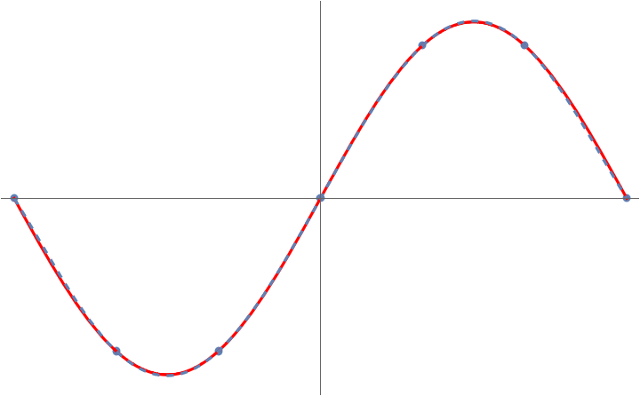
 on the interval
 ![[-1,1]](https://www.ethanepperly.com/wp-content/ql-cache/quicklatex.com-634fe4705a526f221e312cffd3ceda93_l3.png "Rendered by QuickLaTeX.com") :
: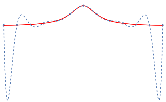
 is terrible! What’s going on? Why doesn’t polynomial interpolation work here? Can we fix it? The answer to the last question is yes and the solution is Chebyshev polynomials.

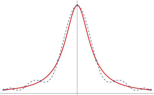
 , like this for ourselves. We’ll assume the interpolation points are given by a function
  so we can form the polynomial interpolant for any desired polynomial degree
  being \textit{injective} so that the points
  are guaranteed to be distinct.
 , the points look like this:
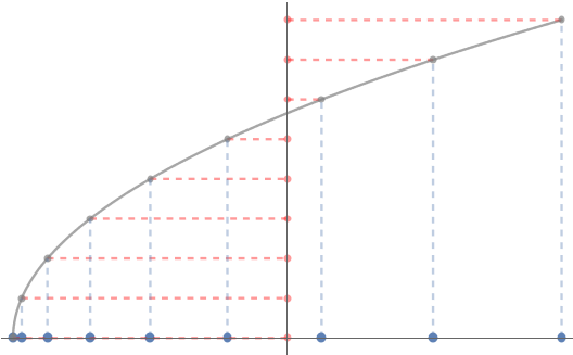

 (shown on horizontal axis)
 .
.
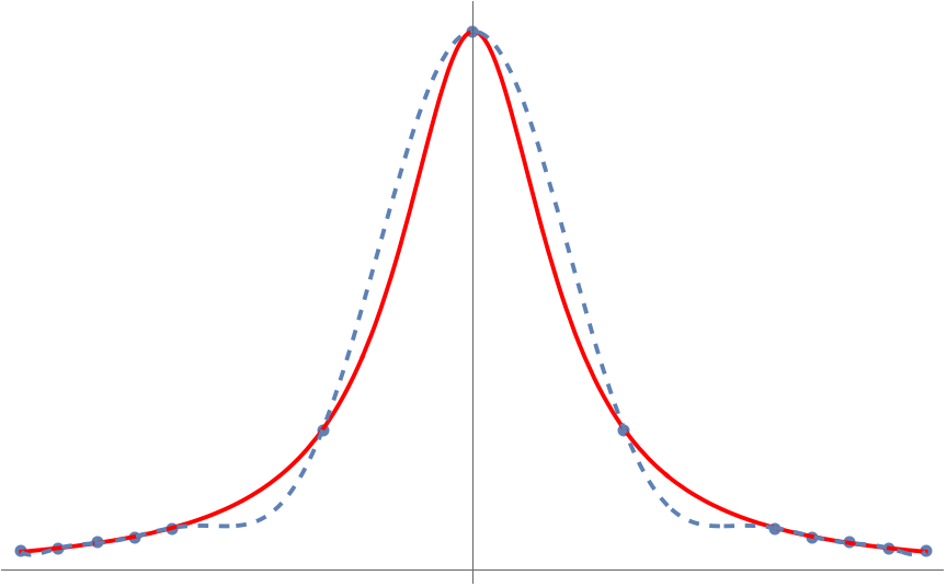
 , we see that these interpolation points now lead to a failure to approximate the function at the middle of the interval, even if we use a lot of interpolation points!
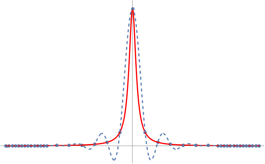
 and
and  are, the more clustered the points will be. For instance,


 , and
, and ,
,  .
. . This function yields points which are more clustered at the endpoints:


 which not too rough (i.e.,
  .
. gives the
  radians along the unit circle. This means that the Chebyshev points are the
  ).
).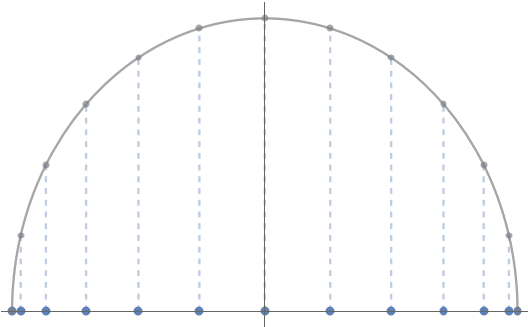
 look like as a function of the angle
  to
to 
 , is a polynomial in the variable
 always take the form

 units of frequency
  units of frequency
  units of frequency
  with exponentially small errors in the number of interpolation points used. By contrast, functions with kinks like
  are approximated with errors which decay much more slowly. See
 is
is  since multiple
  , between which the cosine function is
 , we’ve instead written
 are known as the
  are known as the Chebyshev polynomials
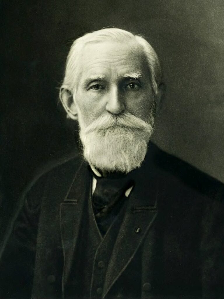

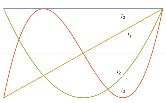
 for
for 
 and
and  are both polynomials, every Chebyshev polynomial is as well.
![\[p^\circ(\theta) = b_n\cos(n\theta) + \cdots + b_1\cos\theta + b_0\]](https://www.ethanepperly.com/wp-content/ql-cache/quicklatex.com-1c6828300bbae5fa0051e7c134da1d61_l3.png "Rendered by QuickLaTeX.com")
![\[p(x) = b_nT_n(x) + \cdots + b_1 T_1(x) + b_0.\]](https://www.ethanepperly.com/wp-content/ql-cache/quicklatex.com-cb291d9f73ebc4e74d0455dac4558a48_l3.png "Rendered by QuickLaTeX.com")
 are orthogonal to each other; are the Chebyshev polynomials?
 matrix
  . That is, we seek to
 of
of  of
of  , our model predicts the output
  is approximately
  . The vector
  is as small as it could possibly be for all choices of coefficient vectors
 . We assume that
  and solve (2) using a linear solver like
  on a computer using a well-designed piece of software, one obtains an approximate solution
  is. The “niceness” of a matrix
  .
. of the largest and smallest
 corresponds to the fact we have roughly 16 decimal digits of accuracy in double precision floating point arithmetic. Thus, if the condition number of
  digits of accuracy in our computed solution.
 . We would hope that we can solve the least squares problem with an accuracy like the rule-of-thumb error bound (3) we had for linear systems of equations, namely a bound like
  . But this is not the kind of accuracy we get for the least squares problem when we solve it using the normal equations. Instead, we get accuracy like
 , then the normal equations give us absolute nonsense for
  times larger than
  . So even if we solve the least squares problem with QR factorization, we still get a squared condition number in our error bound, but this condition number squared is multiplied by the residual
  , which is small if the least squares fit is good. The least squares solution is usually only interesting when the residual is small, thus justifying dropping it in the rule of thumb.
 , etc.
 denote the temperature of the material at point
  . Laplace’s equation states that, at any point

 .
. on the boundary to produce the electric potential
  its boundary. Denote points
  , with the length of
  denoted
  . The double layer potential satisfies
 denotes the directional derivative taken in the direction normal (perpendicular) to the surface at the point
  . Note we choose a unit system for
  at points
 centered at


 square matrix and
  ,
,  in memory and multiplying it with
  .
. .
. . Specifically, our first equation can be rewritten as


 , we have that

 from
from  but, as we did last section, let’s first consider the reverse. To compute


 times equation (8) to equation (7). Following last section, we now instead eliminate
  from equation (8) using equation (7). To do this, we need to integrate equation (7) in order to cancel the integral in equation (8):
 times this integrated equation to equation (8) yields


 using the
 for the
  for the normal vector to
  for the
  for the
  is a so-called
  . Therefore, (9) simplifies to

 for points
 ,
,  is a nonzero constant. Such an integral equation is said to be of the
  ,
,  ,
,  , and
, and  . We say the kernel
 .
. and
and  .
. ):
):
 denote the identity operator on functions: It takes as inputs function
  denote the “integration against
  .
.


 system of linear equations. One can use this as a numerical method to solve second-kind integral equations: First, we
  by a separable kernel of a modest rank
  -decompositions, sparse component analysis, and the blind separation of sums of exponentials
![\[f(t) = a_0 \cos(\omega_0 t - \phi_0) + a_1 \cos(\omega_1 t - \phi_1) + a_2 \cos(\omega_2 t - \phi_2). \]](https://www.ethanepperly.com/wp-content/ql-cache/quicklatex.com-20caba029479063b3c7d59617eff2225_l3.png "Rendered by QuickLaTeX.com")
 ,
,  , and
, and  .
. which we assume are equally spaced
![\[t_j = j\Delta t \quad \textnormal{for} \quad j = 0,1,2,\ldots,n-1.\]](https://www.ethanepperly.com/wp-content/ql-cache/quicklatex.com-4ad3ecc9f18da4793ab2a0113f4afae8_l3.png "Rendered by QuickLaTeX.com")
![\[f_j = f(t_j) \quad \textnormal{for} \quad j = 0,1,2,\ldots,n-1\]](https://www.ethanepperly.com/wp-content/ql-cache/quicklatex.com-2945d5d9092cf48b8b7503194ef8d8e0_l3.png "Rendered by QuickLaTeX.com")
 , where
  it will be helpful to rewrite our formula (1) for
 ![\[\cos \alpha = \frac{\mathrm{e}^{\mathrm{i} \alpha}+\mathrm{e}^{-\mathrm{i} \alpha}}{2}.\]](https://www.ethanepperly.com/wp-content/ql-cache/quicklatex.com-1004ce391e777282f5b1cac7ea69b7b6_l3.png "Rendered by QuickLaTeX.com")
![\[a_0 \cos(\omega_0 t - \phi_0) = d_0 \mathrm{e}^{\mathrm{i} \omega_0t} + d_1 \mathrm{e}^{-\mathrm{i} \omega_0t}.\]](https://www.ethanepperly.com/wp-content/ql-cache/quicklatex.com-b477beb50968f3d0ef261aeafaef89f1_l3.png "Rendered by QuickLaTeX.com")
 and
and  are complex coefficients
  and
and  which contain the same information as the original parameters
  and
and  . Now notice that we are only interest in values
  which are multiples of the spacing
  . Thus, our frequency component can be further rewritten as
![\[a_0 \cos(\omega_0 t_j - \phi_0) = d_0 z_0^j + d_1 z_1^j\]](https://www.ethanepperly.com/wp-content/ql-cache/quicklatex.com-f3728deaec66b4719f2d79377295a1a0_l3.png "Rendered by QuickLaTeX.com")
 and
and  . Performing these reductions, our samples
  take the form
![\[f_j = d_0 z_0^j + d_1 z_1^j + \cdots + d_5 z_5^j. \]](https://www.ethanepperly.com/wp-content/ql-cache/quicklatex.com-80d74d6613b6c1dd28e8e39741fe2043_l3.png "Rendered by QuickLaTeX.com")
 and
and  in the relation (2) from a small number of measurements
  . This can reveal patterns in the sequence which are less obvious when it is represented as given just as numbers. For instance, any seven columns of
  which can be much larger than seven. In addition, as we will soon effectively exploit later, vectors in the nullspace of
 ![\[H = \begin{bmatrix} f_0 & f_1 & f_2 & \cdots & f_{(n-1)/2} \\f_1 & f_2 & f_3 & \cdots & f_{(n-1)/2+1} \\f_2 & f_3 & f_4 & \cdots & f_{(n-1)/2+2} \\\vdots & \vdots & \vdots & \ddots & \vdots \\f_{(n-1)/2} & f{(n-1)/2+1} & f{(n-1)/2+2} & \cdots & f_{n-1} \end{bmatrix}. \]](https://www.ethanepperly.com/wp-content/ql-cache/quicklatex.com-e58f400c13a096efb5c1682c52003056_l3.png "Rendered by QuickLaTeX.com")
 . Observe that the entry in position
  ,
,  . (We use a
  using (2):
![\[H_{ij} = f_{i+j} = \sum_{k=0}^5 d_k z_k^{i+j} = \sum_{k=0}^5 d_k z_k^i \cdot z_k^j. \]](https://www.ethanepperly.com/wp-content/ql-cache/quicklatex.com-c66cda6c8df0e635353009a6469c9d13_l3.png "Rendered by QuickLaTeX.com")
 was just begging to be factorized as
  , which we did. Equation (4) almost looks like the formula for the product of two matrices with entries
  , so it makes sense to introduce the
  matrix
  with entry
  . This is a so-called
 ![\[V = \begin{bmatrix}z_0^0 & z_0^1 & z_0^2 & \cdots & z_0^{(n-1)/2} \\z_1^0 & z_1^1 & z_1^2 & \cdots & z_1^{(n-1)/2} \\\vdots & \vdots & \vdots & \ddots & \vdots \\z_5^0 & z_5^1 & z_5^2 & \cdots & z_5^{(n-1)/2}\end{bmatrix}.\]](https://www.ethanepperly.com/wp-content/ql-cache/quicklatex.com-52248d150045d64416cf49a569abf156_l3.png "Rendered by QuickLaTeX.com")
 diagonal matrix
  , the formula (4) for
  , the factor
 ![\[H = V^\top D V. \]](https://www.ethanepperly.com/wp-content/ql-cache/quicklatex.com-37a707b3000f4e0e2be34695da3f0f68_l3.png "Rendered by QuickLaTeX.com")
 describing our sampled recording
  , determining all the frequencies would be very straightforward.
 of
of ![\[f_m = c_{k-1} f_{m-1} + \cdots + c_1f_{m-k+1}+ c_0 f_{m-k} \quad \textnormal{for every} \quad m = k,\,{k+1},\,{k+2},\cdots. \]](https://www.ethanepperly.com/wp-content/ql-cache/quicklatex.com-f01bd866e8c2df02dc870f3a78958c17_l3.png "Rendered by QuickLaTeX.com")
 because there are six terms in the formula (2) for
  , such a recurrence will allow us to determine the parameters
  . A very good rule of thumb in applied mathematics is to always write down linear equations in matrix–vector notation in see how it looks. Doing this, we obtain
![\[\begin{bmatrix} f_6 \\ f_7 \\ \vdots \\ f_{n-1} \end{bmatrix} = \underbrace{\begin{bmatrix} f_0 & f_1 & f_2 & f_3 & f_4 & f_5 \\ f_1 & f_2 & f_3 & f_4 & f_5 & f_6 \\ \vdots & \vdots & \vdots & \vdots & \vdots & \vdots \\ f_{n-7} & f_{n-6} & f_{n-5} & f_{n-4} & f_{n-3} & f_{n-2} \end{bmatrix}}_{=F}\begin{bmatrix} c_0 \\ c_1 \\ \vdots \\ c_5 \end{bmatrix}. \]](https://www.ethanepperly.com/wp-content/ql-cache/quicklatex.com-7d7dc3e345c47a62fa233007d8d0db69_l3.png "Rendered by QuickLaTeX.com")
 going forward.
 would also be fine for our purposes, but we assume
 ![\[f_{6 \, :\, n-1} = F c, \]](https://www.ethanepperly.com/wp-content/ql-cache/quicklatex.com-b8b53d6de5c09e51040ae688d9bc7d67_l3.png "Rendered by QuickLaTeX.com")
 for the vector on the left-hand side of (7) and collected the recurrence coefficients
  ), the system equations (8) has more equations than unknowns. Fortunately, we are not in the typical case. Despite the fact that we have more equations than unknowns, the linear equations (8) have a unique solution
  In particular, the matrix on the right-hand side of this equation is guaranteed to be nonsingular under our assumptions. Using the Vandermonde decomposition, can you see why?
 ; we seek to find all complex numbers
  gives
gives![\[z^6 = c_0 z^5 + c_1 z^4 + \cdots + c_6. \]](https://www.ethanepperly.com/wp-content/ql-cache/quicklatex.com-4fb9f7123e927dbb902df1eef680ef98_l3.png "Rendered by QuickLaTeX.com")
![\[\begin{bmatrix}f_0 \\ f_1 \\ \vdots \\ f_{n-1}\end{bmatrix} = \begin{bmatrix}1 & 1 & \cdots & 1 \\ z_0 & z_1 & \cdots & z_5 \\ \vdots & \vdots & \ddots & \vdots \\ z_0^{n-1} & z_1^{n-1} & \cdots & z_5^{n-1}\end{bmatrix} \begin{bmatrix}d_0 \\ d_1 \\ \vdots \\ d_{n-1}.\end{bmatrix}. \]](https://www.ethanepperly.com/wp-content/ql-cache/quicklatex.com-4b18fe5a64350989e4534f4b08ef4c23_l3.png "Rendered by QuickLaTeX.com")
 . So far, the benefits of the matrix factorization perspective have yet to really reveal themselves.
 needed to describe the samples and the representation of the samples as a mixture of exponentials is uniquely determined only if the matrix
  ,
,  , and
, and  . (Here, the superscript denotes an index rather than differentiation.) Each signal is a weighted mixture of three sources
  ,
,  , and
, and  , each of which plays a musical chord of three notes (thus representable as a sum of cosines as in (1)). One can think of the sources of being produced three different musical instruments at different places in a room and the recordings
  for each recording
  and form each collection of samples into a Hankel matrix
![\[H^{(\ell)} = \begin{bmatrix} f_0^{(\ell)} & f_1^{(\ell)} & f_2^{(\ell)} & \cdots & f_{(n-1)/2}^{(\ell)} \\f_1^{(\ell)} & f_2^{(\ell)} & f_3^{(\ell)} & \cdots & f_{(n-1)/2+1}^{(\ell)} \\f_2^{(\ell)} & f_3^{(\ell)} & f_4^{(\ell)} & \cdots & f_{(n-1)/2+2}^{(\ell)} \\\vdots & \vdots & \vdots & \ddots & \vdots \\f_{(n-1)/2}^{(\ell)} & f_{(n-1)/2+1}^{(\ell)} & f_{(n-1)/2+2}^{(\ell)} & \cdots & f_{n-1}^{(\ell)} \end{bmatrix}.\]](https://www.ethanepperly.com/wp-content/ql-cache/quicklatex.com-426cddcdbfa1b1bae2c3aaccd49f9974_l3.png "Rendered by QuickLaTeX.com")
 ,
,  , and
, and  as slices of a
  array given by
![\[\mathcal{H}(:,:,\ell) = H^{(\ell)} \quad \textnormal{for} \quad \ell=1,2,3.\]](https://www.ethanepperly.com/wp-content/ql-cache/quicklatex.com-b8b73fa4217e9c667877693a2f3e8348_l3.png "Rendered by QuickLaTeX.com")
![\[H = V^\top DV = \tilde{V}^\top \tilde{D} \tilde{V}\]](https://www.ethanepperly.com/wp-content/ql-cache/quicklatex.com-961c06b840f52d60a6fbc789026074a1_l3.png "Rendered by QuickLaTeX.com")
 can be uniquely determined from the measurements
  rows,
rows,  and perhaps
  ,
,  , etc.
 This matrix has rank-two but no rank-two confluent Vandermonde decomposition. The issue is that when extended to an infinite Hankel matrix
  this (infinite!) matrix has a rank exceeding the size of the original Hankel matrix
  into a Hankel matrix, it can also be useful to form them into a
 ![\[T = \begin{bmatrix} f_{(n-1)/2} & f_{(n-1)/2+1} & f_{(n-1)/2+2} & \cdots & f_{n-1} \\\\f_{(n-1)/2-1} & f_{(n-1)/2} & f_{(n-1)/2+1} & \cdots & f_{n-2} \\\\f_{(n-1)/2-2} & f_{(n-1)/2-1} & f_{(n-1)/2} & \cdots & f_{n-3} \\\\\vdots & \vdots & \vdots & \ddots & \vdots \\\\ f_0 & f_1 & f_2 & \cdots & f_{(n-1)/2} \end{bmatrix}.\]](https://www.ethanepperly.com/wp-content/ql-cache/quicklatex.com-d576130eb33a8d98958a967ae78ae988_l3.png "Rendered by QuickLaTeX.com")
 has the appealing propery that the matrix–vector product
  computes a
 ![\[T = \operatorname{ReversedRows}(V^\top) \cdot DV.\]](https://www.ethanepperly.com/wp-content/ql-cache/quicklatex.com-6cde21a8060919d23383e6cb5fcbaebe_l3.png "Rendered by QuickLaTeX.com")
![\[T = V^* D V,\]](https://www.ethanepperly.com/wp-content/ql-cache/quicklatex.com-ef01b1f93fbb19fa844a5e40b1c8ceb7_l3.png "Rendered by QuickLaTeX.com")
 which are
  where
where  .
.