I’m excited to share that my paper, Fast and forward stable randomized algorithms for linear least-squares problems has been released as a preprint on arXiv.
With the release of this paper, now seemed like a great time to discuss a topic I’ve been wanting to write about for a while: sketching. For the past two decades, sketching has become a widely used algorithmic tool in matrix computations. Despite this long history, questions still seem to be lingering about whether sketching really works:
In this post, I want to take a critical look at the question “does sketching work”? Answering this question requires answering two basic questions:
- What is sketching?
- What would it mean for sketching to work?
I think a large part of the disagreement over the efficacy of sketching boils down to different answers to these questions. By considering different possible answers to these questions, I hope to provide a balanced perspective on the utility of sketching as an algorithmic primitive for solving linear algebra problems.
Sketching
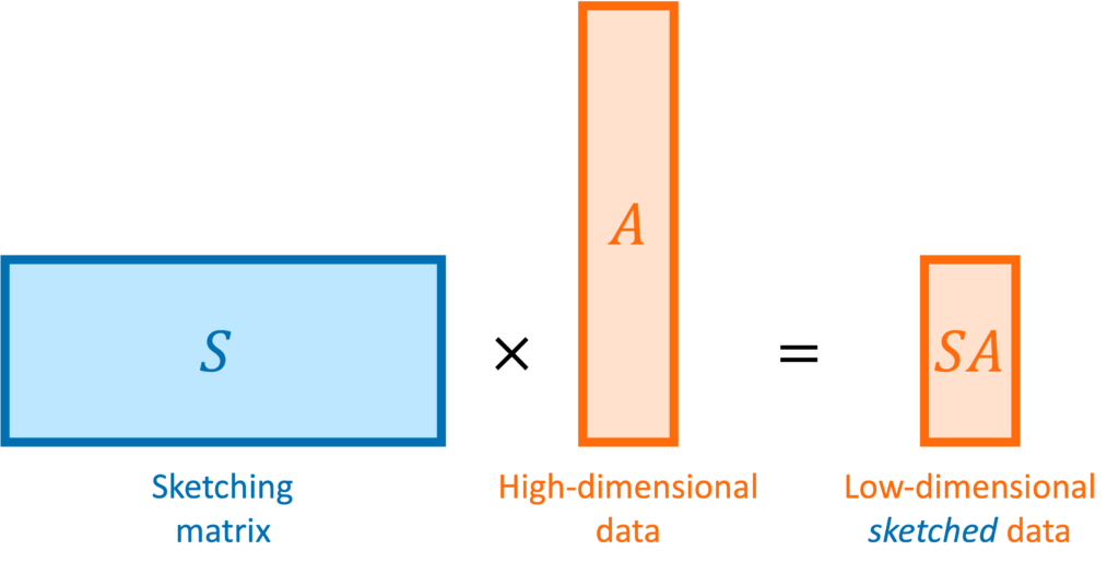
In matrix computations, sketching is really a synonym for (linear) dimensionality reduction. Suppose we are solving a problem involving one or more high-dimensional vectors  or perhaps a tall matrix
  . A sketching matrix is a
  matrix
  where
where  . When multiplied into a high-dimensional vector
  or tall matrix
  , the sketching matrix
  produces compressed or “sketched” versions
  and
and  that are much smaller than the original vector and matrix .
Let  be a collection of vectors. For to be a “good” sketching matrix for
  , we require that preserves the lengths of every vector in up to a distortion parameter
  :
:
(1) ![\[(1-\varepsilon) \norm{x}\le\norm{Sx}\le(1+\varepsilon)\norm{x} \]](https://www.ethanepperly.com/wp-content/ql-cache/quicklatex.com-735df49a45ff5d0bb27d478569004bdd_l3.png "Rendered by QuickLaTeX.com")
for every

in
.
For linear algebra problems, we often want to sketch a matrix . In this case, the appropriate set that we want our sketch to be “good” for is the column space of the matrix , defined to be
![\[\operatorname{col}(A) \coloneqq \{ Ax : x \in \real^k \}.\]](https://www.ethanepperly.com/wp-content/ql-cache/quicklatex.com-5ecde6b43df29caba14fd43682b4cc86_l3.png "Rendered by QuickLaTeX.com")
Remarkably, there exist many sketching matrices that achieve distortion

for

with an output dimension of roughly

. In particular, the sketching dimension

is proportional to the number of columns

of
. This is pretty neat! We can design a single sketching matrix
which preserves the lengths of all infinitely-many vectors

in the column space of
.
Sketching Matrices
There are many types of sketching matrices, each with different benefits and drawbacks. Many sketching matrices are based on randomized constructions in the sense that entries of are chosen to be random numbers. Broadly, sketching matrices can be classified into two types:
- Data-dependent sketches. The sketching matrix is constructed to work for a specific set of input vectors .
- Oblivious sketches. The sketching matrix is designed to work for an arbitrary set of input vectors of a given size (i.e., has
 elements) or dimension ( is a -dimensional linear subspace).
We will only discuss oblivious sketching for this post. We will look at three types of sketching matrices: Gaussian embeddings, subsampled randomized trignometric transforms, and sparse sign embeddings.
The details of how these sketching matrices are built and their strengths and weaknesses can be a little bit technical. All three constructions are independent from the rest of this article and can be skipped on a first reading. The main point is that good sketching matrices exist and are fast to apply: Reducing  to
to  requires roughly
  operations, rather than the
  operations we would expect to multiply a matrix and a vector of length
  .
.
The simplest type of sketching matrix  is obtained by (independently) setting every entry of to be a Gaussian random number with mean zero and variance
  . Such a sketching matrix is called a Gaussian embedding.
Benefits. Gaussian embeddings are simple to code up, requiring only a standard matrix product to apply to a vector or matrix . Gaussian embeddings admit a clean theoretical analysis, and their mathematical properties are well-understood.
Drawbacks. Computing for a Gaussian embedding costs operations, significantly slower than the other sketching matrices we will consider below. Additionally, generating and storing a Gaussian embedding can be computationally expensive.
The subsampled randomized trigonometric transform (SRTT) sketching matrix takes a more complicated form. The sketching matrix is defined to be a scaled product of three matrices
![\[S = \sqrt{\frac{n}{d}} \cdot R \cdot F \cdot D.\]](https://www.ethanepperly.com/wp-content/ql-cache/quicklatex.com-92095cbf9c7d55273bd572a33debe415_l3.png "Rendered by QuickLaTeX.com")
These matrices have the following definitions:
 is a diagonal matrix whose entries are each a random
  (chosen independently with equal probability).
 is a fast trigonometric transform such as a fast discrete cosine transform.
 is a selection matrix. To generate
  , let
, let  be a random subset of
  , selected without replacement. is defined to be a matrix for which
  for every vector .
To store on a computer, it is sufficient to store the diagonal entries of  and the selected coordinates defining . Multiplication of against a vector should be carried out by applying each of the matrices ,
  , and in sequence, such as in the following MATLAB code:
% Generate randomness for S
signs = 2*randi(2,m,1)-3; % diagonal entries of D
idx = randsample(m,d); % indices i_1,...,i_d defining R

% Multiply S against b
c = signs .* b % multiply by D
c = dct(c) % multiply by F
c = c(idx) % multiply by R
c = sqrt(n/d) * c % scale
Benefits. can be applied to a vector in  operations, a significant improvement over the cost of a Gaussian embedding. The SRTT has the lowest memory and random number generation requirements of any of the three sketches we discuss in this post.
Drawbacks. Applying to a vector requires a good implementation of a fast trigonometric transform. Even with a high-quality trig transform, SRTTs can be significantly slower than sparse sign embeddings (defined below). SRTTs are hard to parallelize. In theory, the sketching dimension should be chosen to be  , larger than for a Gaussian sketch.
A sparse sign embedding takes the form
![\[S = \frac{1}{\sqrt{\zeta}} \begin{bmatrix} s_1 & s_2 & \cdots & s_n \end{bmatrix}.\]](https://www.ethanepperly.com/wp-content/ql-cache/quicklatex.com-bb5806806e2e5900d4351c08befbd82e_l3.png "Rendered by QuickLaTeX.com")
Here, each column

is an independently generated random vector with exactly

nonzero entries with random
values in uniformly random positions. The result is a
matrix with only

nonzero entries. The parameter
is often set to a small constant like

in practice.
Benefits. By using a dedicated sparse matrix library, can be very fast to apply to a vector (either  or
or  operations) to apply to a vector, depending on parameter choices (see below). With a good sparse matrix library, sparse sign embeddings are often the fastest sketching matrix by a wide margin.
Drawbacks. To be fast, sparse sign embeddings requires a good sparse matrix library. They require generating and storing roughly  random numbers, higher than SRTTs (roughly numbers) but much less than Gaussian embeddings (
 numbers). In theory, the sketching dimension should be chosen to be and the sparsity should be set to
  ; the theoretically sanctioned sketching dimension (at least according to existing theory) is larger than for a Gaussian sketch. In practice, we can often get away with using
  and
and  .
.
Summary
Using either SRTTs or sparse maps, a sketching a vector of length down to dimensions requires only to operations. To apply a sketch to an entire  matrix thus requires roughly
  operations. Therefore, sketching offers the promise of speeding up linear algebraic computations involving , which typically take
  operations.
How Can You Use Sketching?
The simplest way to use sketching is to first apply the sketch to dimensionality-reduce all of your data and then apply a standard algorithm to solve the problem using the reduced data. This approach to using sketching is called sketch-and-solve.
As an example, let’s apply sketch-and-solve to the least-squares problem:
(2) ![\[\operatorname*{minimize}_{x\in\real^k} \norm{Ax - b}. \]](https://www.ethanepperly.com/wp-content/ql-cache/quicklatex.com-07528304ce875f54aa1173062c5ec10a_l3.png "Rendered by QuickLaTeX.com")
We assume this problem is highly overdetermined with
having many more rows
than columns

.
To solve this problem with sketch-and-solve, generate a good sketching matrix for the set  . Applying to our data and , we get a dimensionality-reduced least-squares problem
(3) ![\[\operatorname*{minimize}_{\hat{x}\in\real^k} \norm{(SA)\hat{x} - Sb}. \]](https://www.ethanepperly.com/wp-content/ql-cache/quicklatex.com-7110d3e9c1dd7e29793603a5bafdd201_l3.png "Rendered by QuickLaTeX.com")
The solution

is the sketch-and-solve solution to the least-squares problem, which we can use as an approximate solution to the original least-squares problem.
Least-squares is just one example of the sketch-and-solve paradigm. We can also use sketching to accelerate other algorithms. For instance, we could apply sketch-and-solve to clustering. To cluster data points  , first apply sketching to obtain
  and then apply an out-of-the-box clustering algorithms like k-means to the sketched data points.
Does Sketching Work?
Most often, when sketching critics say “sketching doesn’t work”, what they mean is “sketch-and-solve doesn’t work”.
To address this question in a more concrete setting, let’s go back to the least-squares problem (2). Let  denote the optimal least-squares solution and let be the sketch-and-solve solution (3). Then, using the distortion condition (1), one can show that
![\[\norm{A\hat{x} - b} \le \frac{1+\varepsilon}{1-\varepsilon} \norm{Ax - b}.\]](https://www.ethanepperly.com/wp-content/ql-cache/quicklatex.com-3d1d034bd8bf93f1c15e435a27a355ee_l3.png "Rendered by QuickLaTeX.com")
If we use a sketching matrix with a distortion of

, then this bound tells us that
(4) ![\[\norm{A\hat{x} - b} \le 2\norm{Ax_\star - b}. \]](https://www.ethanepperly.com/wp-content/ql-cache/quicklatex.com-588170743415f491f48ef2adc3d46628_l3.png "Rendered by QuickLaTeX.com")
Is this a good result or a bad result? Ultimately, it depends. In some applications, the quality of a putative least-squares solution is can be assessed from the residual norm  . For such applications, the bound (4) ensures that is at most twice
  . Often, this means is a pretty decent approximate solution to the least-squares problem.
For other problems, the appropriate measure of accuracy is the so-called forward error  , measuring how close is to . For these cases, it is possible that might be large even though the residuals are comparable (4).
Let’s see an example, using the MATLAB code from my paper:
[A, b, x, r] = random_ls_problem(1e4, 1e2, 1e8, 1e-4); % Random LS problem
S = sparsesign(4e2, 1e4, 8); % Sparse sign embedding
sketch_and_solve = (S*A) \ (S*b); % Sketch-and-solve
direct = A \ b; % MATLAB mldivide
Here, we generate a random least-squares problem of size 10,000 by 100 (with condition number  and residual norm
  ). Then, we generate a sparse sign embedding of dimension
  (corresponding to a distortion of roughly
  ). Then, we compute the sketch-and-solve solution and, as reference, a “direct” solution by MATLAB’s \.
We compare the quality of the sketch-and-solve solution to the direct solution, using both the residual and forward error:
fprintf('Residuals: sketch-and-solve %.2e, direct %.2e, optimal %.2e\n',...
           norm(b-A*sketch_and_solve), norm(b-A*direct), norm(r))
fprintf('Forward errors: sketch-and-solve %.2e, direct %.2e\n',...
           norm(x-sketch_and_solve), norm(x-direct))
Here’s the output:
Residuals: sketch-and-solve 1.13e-04, direct 1.00e-04, optimal 1.00e-04
Forward errors: sketch-and-solve 1.06e+03, direct 8.08e-07
The sketch-and-solve solution has a residual norm of  , close to direct method’s residual norm of
  . However, the forward error of sketch-and-solve is
  nine orders of magnitude larger than the direct method’s forward error of
  .
.
Does sketch-and-solve work? Ultimately, it’s a question of what kind of accuracy you need for your application. If a small-enough residual is all that’s needed, then sketch-and-solve is perfectly adequate. If small forward error is needed, sketch-and-solve can be quite bad.
One way sketch-and-solve can be improved is by increasing the sketching dimension and lowering the distortion . Unfortunately, improving the distortion of the sketch is expensive. Because of the relation  , to decrease the distortion by a factor of ten requires increasing the sketching dimension by a factor of one hundred! Thus, sketch-and-solve is really only appropriate when a low degree of distortion is necessary.
Iterative Sketching: Combining Sketching with Iteration
Sketch-and-solve is a fast way to get a low-accuracy solution to a least-squares problem. But it’s not the only way to use sketching for least-squares. One can also use sketching to obtain high-accuracy solutions by combining sketching with an iterative method.
There are many iterative methods for least-square problems. Iterative methods generate a sequence of approximate solutions  that we hope will converge at a rapid rate to the true least-squares solution, .
To using sketching to solve least-squares problems iteratively, we can use the following observation:
If is a sketching matrix for  , then
  .
.
Therefore, if we compute a QR factorization
![\[SA = QR,\]](https://www.ethanepperly.com/wp-content/ql-cache/quicklatex.com-9edf84077821e9e0cd0c772b77024799_l3.png "Rendered by QuickLaTeX.com")
then
![\[A^\top A \approx (SA)^\top (SA) = R^\top Q^\top Q R = R^\top R.\]](https://www.ethanepperly.com/wp-content/ql-cache/quicklatex.com-90e14ee1172525fd795980cb3ef1a647_l3.png "Rendered by QuickLaTeX.com")
Notice that we used the fact that

since

has orthonormal columns. The conclusion is that

.
Let’s use the approximation to solve the least-squares problem iteratively. Start off with the normal equations
(5) ![\[(A^\top A)x = A^\top b. \]](https://www.ethanepperly.com/wp-content/ql-cache/quicklatex.com-3f3c5265345a169d6633a759854510da_l3.png "Rendered by QuickLaTeX.com")
We can obtain an approximate solution to the least-squares problem by replacing

by

in (5) and solving. The resulting solution is
![\[x_0 = R^{-1} (R^{-\top}(A^\top b)).\]](https://www.ethanepperly.com/wp-content/ql-cache/quicklatex.com-6b63093ea5c1d9714fb0deab43fc4dc3_l3.png "Rendered by QuickLaTeX.com")
This solution  will typically not be a good solution to the least-squares problem (2), so we need to iterate. To do so, we’ll try and solve for the error
  . To derive an equation for the error, subtract
  from both sides of the normal equations (5), yielding
![\[(A^\top A)(x-x_0) = A^\top (b-Ax_0).\]](https://www.ethanepperly.com/wp-content/ql-cache/quicklatex.com-4f1ee993844dbcd8e397f27ccd1deefb_l3.png "Rendered by QuickLaTeX.com")
Now, to solve for the error, substitute
for
again and solve for
, obtaining a new approximate solution

:
![\[x\approx x_1 \coloneqq x_0 + R^{-\top}(R^{-1}(A^\top(b-Ax_0))).\]](https://www.ethanepperly.com/wp-content/ql-cache/quicklatex.com-0496d7e3c8bc117e658c57fc167081be_l3.png "Rendered by QuickLaTeX.com")
We can now go another step: Derive an equation for the error  , approximate
  , and obtain a new approximate solution
  . Continuing this process, we obtain an iteration
(6) ![\[x_{i+1} = x_i + R^{-\top}(R^{-1}(A^\top(b-Ax_i))).\]](https://www.ethanepperly.com/wp-content/ql-cache/quicklatex.com-f8db238fc978e6a8fc968fc5e387ec27_l3.png "Rendered by QuickLaTeX.com")
This iteration is known as the
iterative sketching method. If the distortion is small enough, this method converges at an exponential rate, yielding a high-accuracy least squares solution after a few iterations.
Let’s apply iterative sketching to the example we considered above. We show the forward error of the sketch-and-solve and direct methods as horizontal dashed purple and red lines. Iterative sketching begins at roughly the forward error of sketch-and-solve, with the error decreasing at an exponential rate until it reaches that of the direct method over the course of fourteen iterations. For this problem, at least, iterative sketching gives high-accuracy solutions to the least-squares problem!
To summarize, we’ve now seen two very different ways of using sketching:
- Sketch-and-solve. Sketch the data and and solve the sketched least-squares problem (3). The resulting solution is cheap to obtain, but may have low accuracy.
- Iterative sketching. Sketch the matrix and obtain an approximation
 to . Use the approximation to produce a sequence of better-and-better least-squares solutions
  by the iteration (6). If we run for enough iterations
  , the accuracy of the iterative sketching solution
  can be quite high.
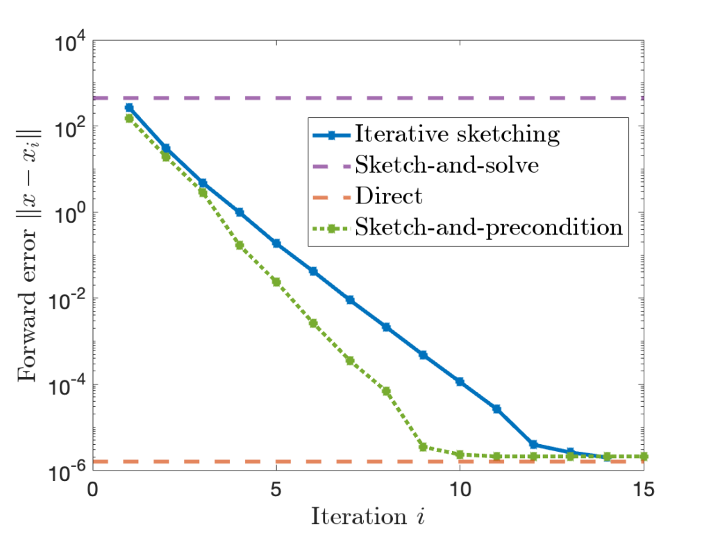
By combining sketching with more sophisticated iterative methods such as conjugate gradient and LSQR, we can get an even faster-converging least-squares algorithm, known as sketch-and-precondition. Here’s the same plot from above with sketch-and-precondition added; we see that sketch-and-precondition converges even faster than iterative sketching does!
“Does sketching work?” Even for a simple problem like least-squares, the answer is complicated:
A direct use of sketching (i.e., sketch-and-solve) leads to a fast, low-accuracy solution to least-squares problems. But sketching can achieve much higher accuracy for least-squares problems by combining sketching with an iterative method (iterative sketching and sketch-and-precondition).
We’ve focused on least-squares problems in this section, but these conclusions could hold more generally. If “sketching doesn’t work” in your application, maybe it would if it was combined with an iterative method.
Just How Accurate Can Sketching Be?
We left our discussion of sketching-plus-iterative-methods in the previous section on a positive note, but there is one last lingering question that remains to be answered. We stated that iterative sketching (and sketch-and-precondition) converge at an exponential rate. But our computers store numbers to only so much precision; in practice, the accuracy of an iterative method has to saturate at some point.
An (iterative) least-squares solver is said to be forward stable if, when run for a sufficient number of iterations, the final accuracy  is comparable to accuracy of a standard direct method for the least-squares problem like MATLAB’s \ command or Python’s scipy.linalg.lstsq. Forward stability is not about speed or rate of convergence but about the maximum achievable accuracy.
The stability of sketch-and-precondition was studied in a recent paper by Meier, Nakatsukasa, Townsend, and Webb. They demonstrated that, with the initial iterate  , sketch-and-precondition is not forward stable. The maximum achievable accuracy was worse than standard solvers by orders of magnitude! Maybe sketching doesn’t work after all?
Fortunately, there is good news:
- The iterative sketching method is provably forward stable. This result is shown in my newly released paper; check it out if you’re interested!
- If we use the sketch-and-solve method as the initial iterate
 for sketch-and-precondition, then sketch-and-precondition appears to be forward stable in practice. No theoretical analysis supporting this finding is known at present.
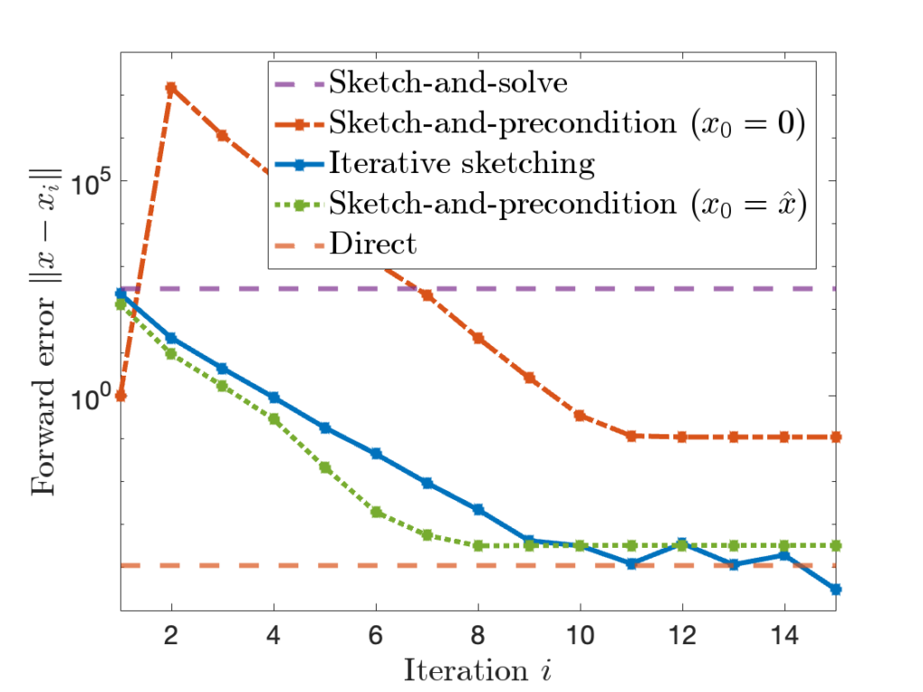
These conclusions are pretty nuanced. To see what’s going, it can be helpful to look at a graph:
The performance of different methods can be summarized as follows: Sketch-and-solve can have very poor forward error. Sketch-and-precondition with the zero initialization is better, but still much worse than the direct method. Iterative sketching and sketch-and-precondition with fair much better, eventually achieving an accuracy comparable to the direct method.
Put more simply, appropriately implemented, sketching works after all!
Conclusion
Sketching is a computational tool, just like the fast Fourier transform or the randomized SVD. Sketching can be used effectively to solve some problems. But, like any computational tool, sketching is not a silver bullet. Sketching allows you to dimensionality-reduce matrices and vectors, but it distorts them by an appreciable amount. Whether or not this distortion is something you can live with depends on your problem (how much accuracy do you need?) and how you use the sketch (sketch-and-solve or with an iterative method).
 of an
of an  matrix
  . The classical method for this purpose is the Girard–Hutchinson estimator
 ![\[\hat{\tr} = \frac{1}{m} \left( x_1^\top Ax_1 + \cdots + x_m^\top Ax_m \right),\]](https://www.ethanepperly.com/wp-content/ql-cache/quicklatex.com-f27a0c05da428b96172a0a8ab23ca54b_l3.png "Rendered by QuickLaTeX.com")
 are independent, identically distributed (iid) random vectors satisfying the isotropy condition
 ![\[\expect[x_ix_i^\top] = I.\]](https://www.ethanepperly.com/wp-content/ql-cache/quicklatex.com-b5ac53011350edc256d9b8c66fdbe7c8_l3.png "Rendered by QuickLaTeX.com")
 ,
,  .
.![\expect[\hat{\tr}] = \tr(A)](https://www.ethanepperly.com/wp-content/ql-cache/quicklatex.com-ad9e9d417b59555f2a6e78e78b6bcbe9_l3.png "Rendered by QuickLaTeX.com") , the variance of
, the variance of  is equal to the mean-square error. Thus, the lowest variance trace estimate is the most accurate. In my previous post on trace estimation, I discussed formulas for the variance
  of the Girard–Hutchinson estimator with different choices of test vectors. In that post, I stated the formulas for different choices of test vectors (Gaussian, random signs, sphere) and showed how those formulas could be proven.
 be the eigenvalues of
 ![\[\overline{\lambda} = \frac{\lambda_1 + \cdots + \lambda_n}{n}.\]](https://www.ethanepperly.com/wp-content/ql-cache/quicklatex.com-3f9e9cf25f6cf20463de5be7e8d40f88_l3.png "Rendered by QuickLaTeX.com")
![\[\Var(\hat{\tr}_{\rm Gaussian}) = \frac{1}{m} \cdot 2 \sum_{i=1}^n \lambda_i^2.\]](https://www.ethanepperly.com/wp-content/ql-cache/quicklatex.com-f8dc441dc68294b0d6ff6af42d3ecef5_l3.png "Rendered by QuickLaTeX.com")
![\[\Var(\hat{\tr}_{\rm sphere}) = \frac{1}{m} \cdot \frac{n}{n+2} \cdot 2\sum_{i=1}^n (\lambda_i - \overline{\lambda})^2.\]](https://www.ethanepperly.com/wp-content/ql-cache/quicklatex.com-6a275f8ba8a47be085e22f679b60b497_l3.png "Rendered by QuickLaTeX.com")
 is smaller than
  by a factor of
  . This improvement is quite minor. Second, and more importantly,
  matrix
  and
and  with a (Haar orthgonal) random matrix of eigenvectors. For simplicity, since the variance of all Girard–Hutchinson estimates is proportional to
  , we take
  . Below show the variance of Girard–Hutchinson estimator for different distributions for the test vector. We see that the sphere distribution leads to a trace estimate which has a variance 300× smaller than the Gaussian distribution. For this example, the sphere and random sign distributions are similar.
 )
)

![\[\Var(\hat{\tr}_{\rm signs}) = 2 \sum_{i\ne j} A_{ij}^2.\]](https://www.ethanepperly.com/wp-content/ql-cache/quicklatex.com-3a6665f8e55563640aedd5ebb0945409_l3.png "Rendered by QuickLaTeX.com")
 depends on the size of the off-diagonal entries of
 ![\[\tr(A) \coloneqq \sum_{i=1}^n A_{ii}.\]](https://www.ethanepperly.com/wp-content/ql-cache/quicklatex.com-80cd9a9ca29d1d3bb13ce28fd80b5e59_l3.png "Rendered by QuickLaTeX.com")
![\[\expect\left[\frac{|\hat{\tr}-\tr(A)|}{\tr(A)}\right] \le \varepsilon \quad \text{using } m= \frac{\rm const}{\varepsilon^2} \text{ matvecs}.\]](https://www.ethanepperly.com/wp-content/ql-cache/quicklatex.com-07898a8a2214416cb97b8b72956e3e76_l3.png "Rendered by QuickLaTeX.com")
 ) requires roughly
  matvecs!
![\[\expect\left[\frac{|\hat{\tr}-\tr(A)|}{\tr(A)}\right] \le \varepsilon \quad \text{using } m= \frac{\rm const}{\varepsilon} \text{ matvecs}.\]](https://www.ethanepperly.com/wp-content/ql-cache/quicklatex.com-b9f186640222c78e5064f83465038b78_l3.png "Rendered by QuickLaTeX.com")
 matvecs to achieve 1% error!
 ![\[\expect\left[\frac{|\hat{\tr}-\tr(A)|}{\tr(A)}\right] \le \varepsilon \quad \text{using } m= \frac{\rm const}{\varepsilon^{0.999}} \text{ matvecs}?\]](https://www.ethanepperly.com/wp-content/ql-cache/quicklatex.com-8bae682300a401dc80869764b302ce8c_l3.png "Rendered by QuickLaTeX.com")
 . The algorithm is allowed to be adaptive: It can use the matvecs
  it has already collected to decide which vector
  to present next. We measure the cost of the algorithm in terms of the number of matvecs alone, and the algorithm knows nothing about the psd matrix
  and
and  with up to
  . Then
  would be an allowed input vector, but
  would not be (too many digits after the decimal place). Similarly,
  would not be valid because its entries exceed
  . For this analysis of trace estimation, we use
  (no powers of ten allowed)!
![\[\expect\left[\frac{|\hat{\tr}-\tr(A)|}{\tr(A)}\right] \le \varepsilon \quad \text{using } m= \frac{\rm const}{\varepsilon^{0.999}} \text{ matvecs}.\]](https://www.ethanepperly.com/wp-content/ql-cache/quicklatex.com-9034edba9bafb68809d24d54f5a830e6_l3.png "Rendered by QuickLaTeX.com")
 , and they are interested in computing a function
  of both their inputs.
 with
with  and
and ![\[\text{Case 0: } x^\top y \ge\sqrt{n} \quad \text{or} \quad \text{Case 1: } x^\top y \le -\sqrt{n}. \]](https://www.ethanepperly.com/wp-content/ql-cache/quicklatex.com-3134941eeedf133f83ba4795b499332f_l3.png "Rendered by QuickLaTeX.com")
 , determines whether they are in case 0 or case 1, and sends Bob a single bit to communicate the answer. This procedure requires
  bits of communication.
 probability for every pair of inputs
  bits of communication.
 and
and  . For the less familiar, it can be helpful to interpret
  , and consider (but do not form!) the positive semidefinite matrix
 ![\[A = (X+Y)^\top (X+Y).\]](https://www.ethanepperly.com/wp-content/ql-cache/quicklatex.com-2b1df104e3d571430963573b54d5c4df_l3.png "Rendered by QuickLaTeX.com")
![\[\tr(A) = \tr(X^\top X) + 2\tr(X^\top Y) + \tr(Y^\top Y) = 2n + 2(x^\top y).\]](https://www.ethanepperly.com/wp-content/ql-cache/quicklatex.com-a0f6e916740a9c27733c659418cc15cf_l3.png "Rendered by QuickLaTeX.com")
 :
:![\[\text{Case 0: } \tr(A)\ge 2n + 2\sqrt{n} \quad \text{or} \quad \text{Case 1: } \tr(A) \le 2n-2\sqrt{n}. \]](https://www.ethanepperly.com/wp-content/ql-cache/quicklatex.com-1fea970636b48c827e4584d3655b9e3c_l3.png "Rendered by QuickLaTeX.com")
 or
or  ) and sends the result to Bob.
 for some vector
  with entries between
  whose entries are integers between
  and
and  . Since
  , interconverting between
  is trivial. Alice and Bob’s procedure for computing
  .
. and sends it to Alice.
 and sends it to Bob.
 , Bob computes
  and sends its to Alice.
 .
. and
and  are
are  and have
  and
and  . We conclude the communication cost for one matvec is
  bits.
bits. , BestTraceAlgorithm requires at most
  matvecs and, for any positive semidefinite input matrix
 ![\[\expect\left[\frac{|\hat{\tr}-\tr(A)|}{\tr(A)}\right] \le \varepsilon.\]](https://www.ethanepperly.com/wp-content/ql-cache/quicklatex.com-a9165ea3846d540eb654af9f7f59a5c2_l3.png "Rendered by QuickLaTeX.com")
 matvecs.
![\[\left| \frac{\hat{\tr} - \tr(A)}{\tr(A)} \right| \le \frac{1}{\sqrt{n}},\]](https://www.ethanepperly.com/wp-content/ql-cache/quicklatex.com-8327e1b03c9ba9162fb737e40a192b3a_l3.png "Rendered by QuickLaTeX.com")
 bits. Chakrabati and Regev showed that Gap-Hamming requires
  bits of communication (for some
  ) to solve the Gap-Hamming problem with
  , then Alice and Bob fail to solve the Gap-Hamming problem with at least
  probability. Thus,
 ![\[\text{If } m < \frac{cn}{T} = \Theta\left( \frac{\sqrt{n}}{b+\log n} \right), \quad \text{then } \left| \frac{\hat{\tr} - \tr(A)}{\tr(A)} \right| > \frac{1}{\sqrt{n}} \text{ with probability at least } \frac{1}{3}.\]](https://www.ethanepperly.com/wp-content/ql-cache/quicklatex.com-74364fd915239fdaf0889d005378b7ba_l3.png "Rendered by QuickLaTeX.com")
![\[\text{If }\left| \frac{\hat{\tr} - \tr(A)}{\tr(A)} \right| \le \frac{1}{\sqrt{n}}\text{ with probability at least } \frac{2}{3}, \quad \text{then } m \ge \Theta\left( \frac{\sqrt{n}}{b+\log n} \right).\]](https://www.ethanepperly.com/wp-content/ql-cache/quicklatex.com-81fbd6e8e08c9759a6cbf5ac4f9782e2_l3.png "Rendered by QuickLaTeX.com")
 . Then, by (3) and
 ![\[\left| \frac{\hat{\tr} - \tr(A)}{\tr(A)} \right| \le \frac{1}{\sqrt{n}} \quad \text{with probability at least }\frac{2}{3}.\]](https://www.ethanepperly.com/wp-content/ql-cache/quicklatex.com-95db791999f5573659f14f5b0d4a386e_l3.png "Rendered by QuickLaTeX.com")
![\[m \ge \Theta\left( \frac{\sqrt{n}}{b+\log n} \right) \text{ matvecs}.\]](https://www.ethanepperly.com/wp-content/ql-cache/quicklatex.com-8f0975698051029d6273269409146a9f_l3.png "Rendered by QuickLaTeX.com")
 , we conclude that any trace estimation algorithm, even BestTraceAlgorithm, requires
![\[m \ge \Theta \left( \frac{1}{\varepsilon (b+\log(1/\varepsilon))} \right) \text{ matvecs}.\]](https://www.ethanepperly.com/wp-content/ql-cache/quicklatex.com-b3eb651ca114a7fe19f3b8c5d3e64063_l3.png "Rendered by QuickLaTeX.com")
 matvecs. This proves the MMMW theorem.
 be a domain and let
  be a (
 . We consider the task of evaluating
 ![\[I[f] = \int_\Omega f(x) g(x) \, \mathrm{d}\mu(x).\]](https://www.ethanepperly.com/wp-content/ql-cache/quicklatex.com-4767401252e7558c87b5a518f3609468_l3.png "Rendered by QuickLaTeX.com")
 ,
, ![I[f]](https://www.ethanepperly.com/wp-content/ql-cache/quicklatex.com-603f22dedcf932b6f47e37160c09afd8_l3.png "Rendered by QuickLaTeX.com") for multiple different functions
for multiple different functions  .
.
![\[\hat{I}_{w,s}[f] = \sum_{i=1}^n w_i f(s_i) \approx I[f].\]](https://www.ethanepperly.com/wp-content/ql-cache/quicklatex.com-4bb6a83827b630719dd50338a790b9c6_l3.png "Rendered by QuickLaTeX.com")
 and points
  such that the approximation
 ![\hat{I}_{w,s}[f] \approx I[f]](https://www.ethanepperly.com/wp-content/ql-cache/quicklatex.com-61580a8cc2043483ce9c1ab09e3ea85e_l3.png "Rendered by QuickLaTeX.com") is accurate.
is accurate.
 be an RKHS with
  . We can interpret the norm as assigning a roughness
  to each function
  . It is related to the RKHS
  by the reproducing property
![\[f(x)=\langle f, k(x,\cdot)\rangle \quad \text{for every }f\in\mathcal{H},x\in\Omega.\]](https://www.ethanepperly.com/wp-content/ql-cache/quicklatex.com-276db3513a1ea34da49f342ad7f4a7ea_l3.png "Rendered by QuickLaTeX.com")
 represents the univariate function obtained by setting the first input of
  . Let’s first assume that the nodes
  are fixed, and talk about how to pick the weights
  that we’ll called the ideal weights. There (at least) are five equivalent ways of characterizing the ideal weights. We’ll present all of them. As an exercise, you can try and convince yourself that these characterizations are equivalent, giving rise to the same weights.
 .
.![\[\hat{I}_{w_\star,s}[k(s_i,\cdot)]=I[k(s_i,\cdot)] \quad \text{for } i=1,2,\ldots,n.\]](https://www.ethanepperly.com/wp-content/ql-cache/quicklatex.com-52bf51e5f4ddb42195d5896ff71ebe02_l3.png "Rendered by QuickLaTeX.com")
 :
:![\[\sum_{j=1}^n k(s_i,s_j)w^\star_j = \int_\Omega k(s_i,x) g(x)\,\mathrm{d}\mu(x) \quad \text{for }i=1,2,\ldots,n.\]](https://www.ethanepperly.com/wp-content/ql-cache/quicklatex.com-1a5ca36966f56dae9d994e208f9ef036_l3.png "Rendered by QuickLaTeX.com")
 is the ideal weights.
 at the nodes, obtaining an interpolant
  . Then, obtain an approximation to the integral by integrating the interpolant:
![\[\hat{I}_{w^\star,s}[f] \coloneqq \int_\Omega \hat{f}(x) g(x) \, \mathrm{d}\mu(x).\]](https://www.ethanepperly.com/wp-content/ql-cache/quicklatex.com-0c68060fdf085f41d9cbdd9cc5c16e31_l3.png "Rendered by QuickLaTeX.com")
![\[\hat{f} = \argmin \{ \norm{h} : h(s_i) = f(s_i) \text{ for } i=1,\ldots,n\}.\]](https://www.ethanepperly.com/wp-content/ql-cache/quicklatex.com-5619a986180c554d2a079e5156a97571_l3.png "Rendered by QuickLaTeX.com")
![\[\hat{f} = \sum_{i=1}^n \alpha_i k(\cdot,s_i)\]](https://www.ethanepperly.com/wp-content/ql-cache/quicklatex.com-0abcded0eda92deac99b904817afdf5b_l3.png "Rendered by QuickLaTeX.com")
 .With a little algebra, you can show that the integral of
 ![\[I[\hat{f}] = \sum_{i=1}^n w^\star_i f(s_i),\]](https://www.ethanepperly.com/wp-content/ql-cache/quicklatex.com-f0da23bc7dc97894b0a6702b6bf6ddfb_l3.png "Rendered by QuickLaTeX.com")
![\[\operatorname{Err}(w,s)=\sup_{\norm{f}\le 1}\left| I[f] - \hat{I}_{w,s}[f]\right|.\]](https://www.ethanepperly.com/wp-content/ql-cache/quicklatex.com-6e46307dc4cdac54a3ab010b36ed7858_l3.png "Rendered by QuickLaTeX.com")
 is the highest possible quadrature error for a function
  of norm at most 1.
![\[w^\star=\operatorname*{argmin}_{w\in\real^n}\operatorname{Err}(w,s).\]](https://www.ethanepperly.com/wp-content/ql-cache/quicklatex.com-06e68886b8279d9d592cae3775d4295f_l3.png "Rendered by QuickLaTeX.com")
 for a mean-zero Gaussian process with
 ![\[\Cov(f(x),f(y))=k(x,y)\quad \text{for every } x,y\in\Omega.\]](https://www.ethanepperly.com/wp-content/ql-cache/quicklatex.com-19fea8ea8406c891c0d6bab2166dc4a4_l3.png "Rendered by QuickLaTeX.com")
![\[\operatorname{MSE}(w,s)\coloneqq \expect_{f\sim\operatorname{GP}(0,k)} \left( I[f] - \hat{I}_{w,s}[f] \right)^2.\]](https://www.ethanepperly.com/wp-content/ql-cache/quicklatex.com-4741e0bcba7276b0a3a9266cd61b54c0_l3.png "Rendered by QuickLaTeX.com")
![\[\operatorname{MSE}(w,s)=\operatorname{Err}(w,s)^2.\]](https://www.ethanepperly.com/wp-content/ql-cache/quicklatex.com-dc387f1211b9e5a070f2778a8205c022_l3.png "Rendered by QuickLaTeX.com")
![\[w^\star=\operatorname*{argmin}_{w\in\real^n}\operatorname{MSE}(w,s).\]](https://www.ethanepperly.com/wp-content/ql-cache/quicklatex.com-32506adbc7176da52a920dbf4c373149_l3.png "Rendered by QuickLaTeX.com")
 . The integral of this random function
 ![I[h]](https://www.ethanepperly.com/wp-content/ql-cache/quicklatex.com-e47eba0764d69669e85367cf245d71d3_l3.png "Rendered by QuickLaTeX.com") is a random variable. To numerically integrate a function
is a random variable. To numerically integrate a function  agreeing with
 ![\[\hat{I}_{w^\star,s}[f]\coloneqq \expect_{h\sim\operatorname{GP}(0,k)}[I[h] \mid h(s_i)=f(s_i) \text{ for } i=1,\ldots,n].\]](https://www.ethanepperly.com/wp-content/ql-cache/quicklatex.com-ce1156fb9da612607ae0158770a34645_l3.png "Rendered by QuickLaTeX.com")
 , it is reasonable to add an additional constraint that the weights
 ![\[w\in\Delta\coloneqq \left\{ p\in\real^n_+ : \sum_{i=1}^n p_i = 1\right\}.\]](https://www.ethanepperly.com/wp-content/ql-cache/quicklatex.com-55c593b2593abc9ea8c18d4f8edbccd3_l3.png "Rendered by QuickLaTeX.com")
 ; thus, in effect, quadrature amounts to approximating one probability measure
  . Additional constraints such as these can easily be imposed when using the optimization characterizations 3 and 4 of the ideal weights. See
  ? To pick the nodes, it seems sensible to try and minimize the worst-case error
  with the ideal weights
 ![\[\operatorname{Err}(w^\star,s) = \norm{\int_\Omega (k(\cdot,x) - \hat{k}_s(\cdot,x)) g(x) \, \mathrm{d}\mu(x)}.\]](https://www.ethanepperly.com/wp-content/ql-cache/quicklatex.com-f66a0cdfc8a943a944dad0fed98dbad9_l3.png "Rendered by QuickLaTeX.com")
 is the
 ![\[\hat{k}_s(x,y) = k(x,s) k(s,s)^{-1} k(s,y).\]](https://www.ethanepperly.com/wp-content/ql-cache/quicklatex.com-9c55d13be5a7cdb27139303cb08ec19f_l3.png "Rendered by QuickLaTeX.com")
 for the kernel matrix with
  entry
entry  and
and  and
and  for the row and column vectors with
  th entry
  and
and  .
.
 as accurate as possible.
 is and, thus, the smaller the error
  , it has a high probability of placing the next node
  far from the previously selected nodes.
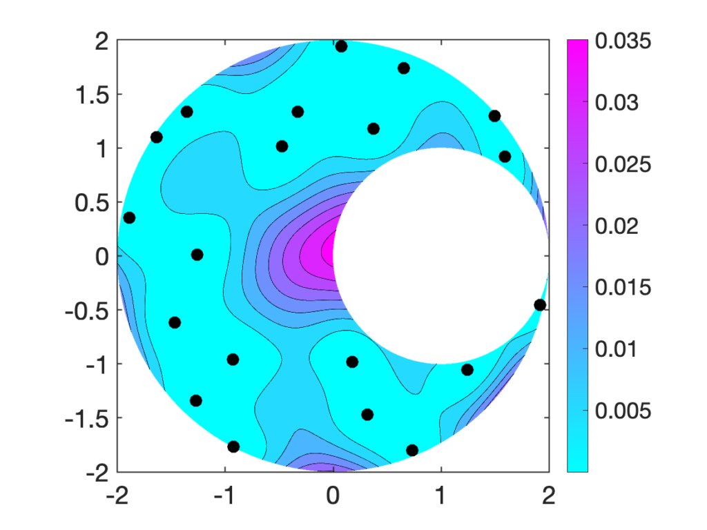
 or vector
 ![\[(1-\varepsilon) \norm{x} \le \norm{Sx} \le (1+\varepsilon) \norm{x} \quad \text{for every } x \in \operatorname{col}(A).\]](https://www.ethanepperly.com/wp-content/ql-cache/quicklatex.com-06811a2d05bdccddd7b3c3079ed47729_l3.png "Rendered by QuickLaTeX.com")
 denotes the
  matrix.
 (one million) and output dimension
  .
.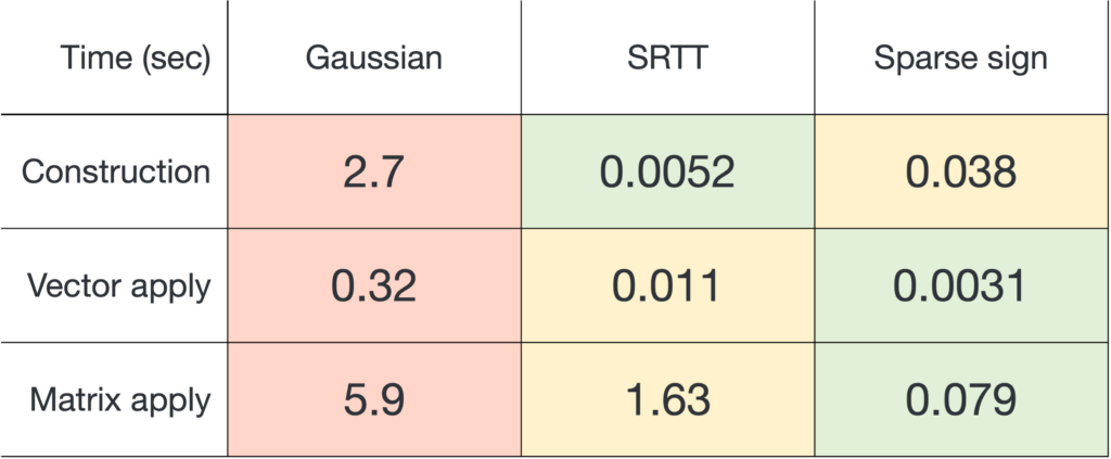
 and applying it to a matrix
  , sparse sign embeddings are 14× faster than SRTTs and 73× faster than Gaussian embeddings.
 and
and  using the MATLAB
  (equivalently,
  ) is shown as a dashed line.
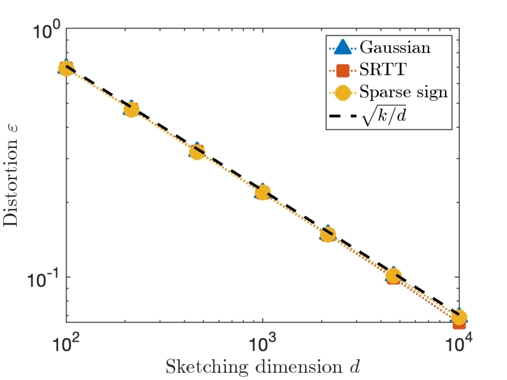
 is taken to be a matrix with independent standard Gaussian random values.
 is taken to be the
  is taken to be the
  identity matrix stacked onto a
  matrix of zeros.
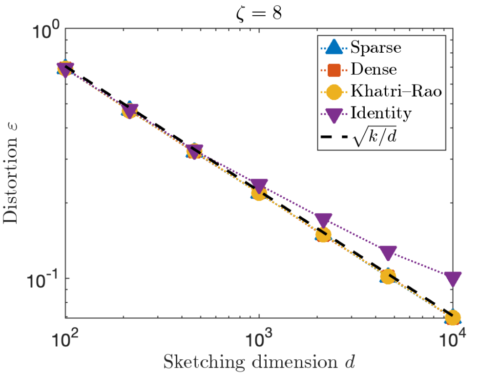
 . However, for the last test matrix “Identity”, we see the distortion begins to slightly exceed this predicted distortion for
  .
. , we can increase the value of the sparsity parameter
 ![\[\zeta = \max \left( 8 , \left\lceil 2\sqrt{\frac{d}{k}} \right\rceil \right).\]](https://www.ethanepperly.com/wp-content/ql-cache/quicklatex.com-5f1ebe7695d9918399b0f97b628fcce1_l3.png "Rendered by QuickLaTeX.com")
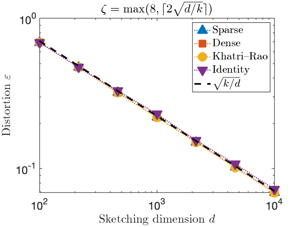
 can be necessary to achieve the optimal distortion.
![\[S = \frac{1}{\sqrt{\zeta}} \begin{bmatrix} s_1 & \cdots & s_n \end{bmatrix}.\]](https://www.ethanepperly.com/wp-content/ql-cache/quicklatex.com-4871e53b2bb59ad11946f2d1eafc66f7_l3.png "Rendered by QuickLaTeX.com")
![\[(1-\varepsilon) \norm{x} \le \norm{Sx} \le (1+\varepsilon) \norm{x} \quad \text{for all }x \in \operatorname{col}(A).\]](https://www.ethanepperly.com/wp-content/ql-cache/quicklatex.com-41fd14292c1c85cd318dde801a75e1bd_l3.png "Rendered by QuickLaTeX.com")
![\[d = \frac{k}{\varepsilon^2} \quad \text{and} \quad \zeta = \max\left(8,\frac{2}{\varepsilon}\right).\]](https://www.ethanepperly.com/wp-content/ql-cache/quicklatex.com-ed85cec8dadffec7c7a3b4e099d6637d_l3.png "Rendered by QuickLaTeX.com")
 . The value
  has demonstrated deficiencies and should almost always be avoided (see below). The scaling
 ![\[d = \mathcal{O} \left( \frac{k \log k}{\varepsilon^2} \right) \quad \text{and} \quad \zeta = \mathcal{O}\left( \frac{\log k}{\varepsilon} \right).\]](https://www.ethanepperly.com/wp-content/ql-cache/quicklatex.com-4fb6d0d60c85bc8a60d95bb0a19e63d6_l3.png "Rendered by QuickLaTeX.com")
 factor and the lack of explicit constants in the
  and can also be generated using a single line. The real challenge to generating sparse sign embeddings in MATLAB is the row indices, since each batch of
  sparse sign embedding with sparsity
  and weights
  . To apply
 ![\[b \in \real^n \longmapsto Sb = (w_1 b_{i_1},\ldots,w_db_{i_d}) \in \real^d.\]](https://www.ethanepperly.com/wp-content/ql-cache/quicklatex.com-712b97fc6f6efb9bf9a40dac2a652f5c_l3.png "Rendered by QuickLaTeX.com")
 for the hard “Identity” test matrix used above.
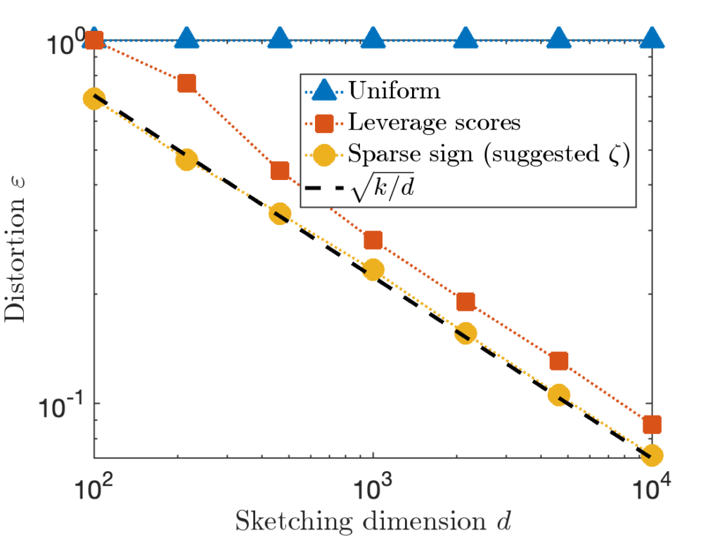
 for each row of
  , and compare the distortion of CountSketch to the sparse sign embedding with parameters
  :
: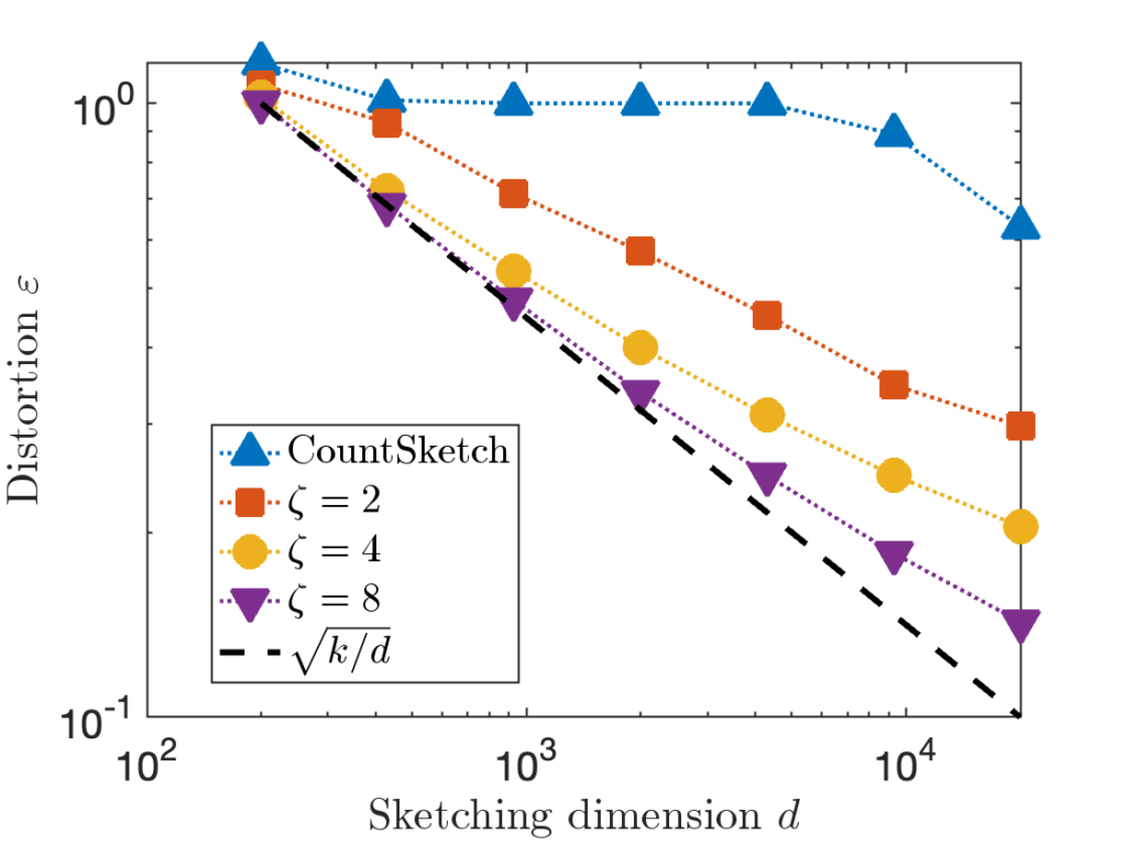
 , 20× higher than
  in order to achieve distortion
  (or perhaps
  ). This difference between
  for CountSketch and
  for other sketching matrices is a at the root of CountSketch’s woefully bad performance on some inputs.
 is an informal symbol meaning “proportional to”.
 . This is Theorem 16 in
  , where
  is a CountSketch of size
  and
and  is a Gaussian sketching matrix of size
  .
. , then the distortion of
  with high probability.
![\[SA = \begin{bmatrix} s_1 & \cdots & s_k \end{bmatrix}\]](https://www.ethanepperly.com/wp-content/ql-cache/quicklatex.com-82c7ea0e5c52b6bd9bdb389f3d3f92d7_l3.png "Rendered by QuickLaTeX.com")
 has a single
  in a uniformly random location
  .
.
 are not all different from each other, say
  . Set
. Set  , where
  is the standard basis vector with
  but
but  . Thus, for the distortion relation
 ![\[(1-\varepsilon) \norm{x} =(1-\varepsilon)\sqrt{2} \le 0 = \norm{(SA)x}\]](https://www.ethanepperly.com/wp-content/ql-cache/quicklatex.com-b08feebb30829a0e73b02188eba6f901_l3.png "Rendered by QuickLaTeX.com")
 . Thus,
 ![\[\prob \{ \varepsilon \ge 1 \} \ge \prob \{ j_1,\ldots,j_k \text{ are not distinct} \}.\]](https://www.ethanepperly.com/wp-content/ql-cache/quicklatex.com-12fa7b716b97c7e9482f4f6327bd4728_l3.png "Rendered by QuickLaTeX.com")
 pairs of people. Each pair of people has a
  chance of sharing a birthday, so the expected number of birthdays in a room of 23 people is
  . Since are 0.69 birthdays shared on average in a room of 23 people, it is perhaps less surprising that 23 is the critical number at which the chance of two people sharing a birthday exceeds 50%.
 and
and  in CountSketch have a
  pairs of indices, so the expected number of equal indices
  . Thus, we should anticipate
  is required to ensure that
 ![\[\prob \{ j_1,\ldots,j_k \text{ are not distinct} \} = 1 - \prob \{ j_1,\ldots,j_k \text{ are distinct} \}.\]](https://www.ethanepperly.com/wp-content/ql-cache/quicklatex.com-338a38501a565185b794f8ed03803c9a_l3.png "Rendered by QuickLaTeX.com")
 are all distinct, the probability
  are distinct is just the probability that
  values
 ![\[\prob\{ j_1,\ldots,j_i \text{ are distinct} \mid j_1,\ldots,j_{i-1} \text{ are distinct}\} = 1 - \frac{i-1}{d}.\]](https://www.ethanepperly.com/wp-content/ql-cache/quicklatex.com-b474f00c44e53b7c3c398d56121e1ac3_l3.png "Rendered by QuickLaTeX.com")
![\[\prob \{ j_1,\ldots,j_k \text{ are distinct} \} = \prod_{i=1}^k \left(1 - \frac{i-1}{d} \right).\]](https://www.ethanepperly.com/wp-content/ql-cache/quicklatex.com-7dd28281f8dbed8b3a1452a21e7410c8_l3.png "Rendered by QuickLaTeX.com")
 for every
  , obtaining
![\[\mathbb{P} \{ j_1,\ldots,j_k \text{ are distinct} \} \le \prod_{i=0}^{k-1} \exp\left(-\frac{i}{d}\right) = \exp \left( -\frac{1}{d}\sum_{i=0}^{k-1} i \right) = \exp\left(-\frac{k(k-1)}{2d}\right).\]](https://www.ethanepperly.com/wp-content/ql-cache/quicklatex.com-8d9d4c7d12af0fd89e53ca261c5df287_l3.png "Rendered by QuickLaTeX.com")
![\[\prob \{ \varepsilon \ge 1 \} \ge 1-\prob \{ j_1,\ldots,j_k \text{ are distinct} \\}\ge 1-\exp\left(-\frac{k(k-1)}{2d}\right).\]](https://www.ethanepperly.com/wp-content/ql-cache/quicklatex.com-144cfc73d778c4f9ed7442f5a6610e5e_l3.png "Rendered by QuickLaTeX.com")
![\[\prob\{\varepsilon \ge 1\} \ge \frac{1}{2} \quad \text{if} \quad d \le \frac{k(k-1)}{2\ln 2}.\]](https://www.ethanepperly.com/wp-content/ql-cache/quicklatex.com-e11567078a415b79b06a8e5e6f0b1600_l3.png "Rendered by QuickLaTeX.com")
 is
is  at every iteration. Later,
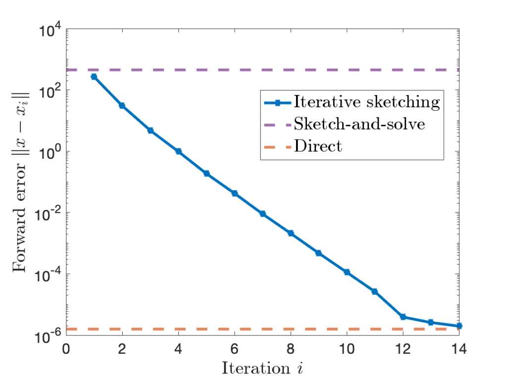
 and residual
  .
.
![\[\chi^2\left(\rho^{(n)} \, \middle|\middle| \, \pi\right) \le \left( \max \{ \lambda_2, -\lambda_n \} \right)^{2n} \chi^2\left(\rho^{(0)} \, \middle|\middle| \, \pi\right).\]](https://www.ethanepperly.com/wp-content/ql-cache/quicklatex.com-ed65d0043f7a436b0f42a6d096d34e9f_l3.png "Rendered by QuickLaTeX.com")
 denotes the distribution of the chain at time
  denotes the
  denotes the
 denote the decreasingly ordered
  . To bound the rate of convergence to stationarity, we therefore must upper bound
  and lower bound
  .
.
 Fortunately, there is a trick.
 for every
  , where
  denotes the identity matrix. It is easy to see that the stationary distribution
  :
:![\[\pi^\top P^{\rm lazy} = \frac{1}{2} \pi^\top P + \frac{1}{2} \pi^\top I = \frac{1}{2} \pi^\top + \frac{1}{2} \pi^\top = \pi^\top.\]](https://www.ethanepperly.com/wp-content/ql-cache/quicklatex.com-d33d9a3024c655134a56d89b119cf39c_l3.png "Rendered by QuickLaTeX.com")
![\[\lambda_i^{\rm lazy} = \frac{1+\lambda_i}{2}.\]](https://www.ethanepperly.com/wp-content/ql-cache/quicklatex.com-ac2938aa6854a708a394222649af1e66_l3.png "Rendered by QuickLaTeX.com")
 are
are  , all of the eigenvalues of the lazy chain are
  . Thus, the smallest eigenvalue of
  :
:![\[\chi^2\left(\rho^{(n)} \, \middle|\middle| \, \pi\right) \le \left( \lambda_2^{\rm lazy} \right)^{2n} \chi^2\left(\rho^{(0)} \, \middle|\middle| \, \pi\right).\]](https://www.ethanepperly.com/wp-content/ql-cache/quicklatex.com-861a132f08a1c2b208d61eb004ed58bb_l3.png "Rendered by QuickLaTeX.com")
 over a random variable
  drawn from the stationary distribution:
 ![\[\expect_{x\sim \pi} [f(x)] = \sum_{i=1}^m f(i) \pi_i.\]](https://www.ethanepperly.com/wp-content/ql-cache/quicklatex.com-6399c58f0e1b13f3cffac439c145d3b4_l3.png "Rendered by QuickLaTeX.com")
 of the value of
  values
  of the chain
![\[\hat{f}_{N}\coloneqq \frac{1}{N}\sum_{n=0}^{N-1} f(x_i).\]](https://www.ethanepperly.com/wp-content/ql-cache/quicklatex.com-591e83a4f5551f6826ddffb5de03ce72_l3.png "Rendered by QuickLaTeX.com")
![\[\hat{f}_N = \frac{1}{N}\sum_{n=0}^{N-1} f(x_i)\]](https://www.ethanepperly.com/wp-content/ql-cache/quicklatex.com-615239005583b665db04e6a578abec08_l3.png "Rendered by QuickLaTeX.com")
 denote the states of a Markov chain initialized in the stationary distribution
  . For a large number
 ![\expect_{x\sim \pi} [f(x)]](https://www.ethanepperly.com/wp-content/ql-cache/quicklatex.com-e4b2ff50078922c10c1f0a32237a19d6_l3.png "Rendered by QuickLaTeX.com") and variance
and variance  where
where ![\[\sigma^2 = \Var[f(x_0)] + 2\sum_{n=1}^\infty \Cov(f(x_0),f(x_n)). \]](https://www.ethanepperly.com/wp-content/ql-cache/quicklatex.com-b209aff956ed442df57ac781c0376a2f_l3.png "Rendered by QuickLaTeX.com")
 and later values
  . The faster the covariance decreases, the smaller
  will be and thus the smaller the error for the Markov chain average.
 ,
, ![\[\frac{\hat{f}_N - \expect_{x \sim \pi} [f(x)]}{\sqrt{N}}\]](https://www.ethanepperly.com/wp-content/ql-cache/quicklatex.com-f5818a8980215e63da79048168aa8b79_l3.png "Rendered by QuickLaTeX.com")
 be any function.
 that are
 ![\[\langle \varphi_i,\varphi_j \rangle = \expect_{x\sim \pi} [\varphi_i(x)\varphi_j(x)] = \begin{cases}1, & i = j, \\0, & i \ne j.\end{cases}\]](https://www.ethanepperly.com/wp-content/ql-cache/quicklatex.com-139934705e34440f3c903f0e089f580b_l3.png "Rendered by QuickLaTeX.com")
 as defining a function
  . Thus, we can expand the function
 ![\[f = c_1 \varphi_1 + \cdots + c_m \varphi_m. \]](https://www.ethanepperly.com/wp-content/ql-cache/quicklatex.com-c7d7e27ce6d2d6d0e3c721a120eef469_l3.png "Rendered by QuickLaTeX.com")
 is the vector of all ones (or, equivalently, the function that outputs
  at time
  at time
  ?
? conditional on the chain starting at
  :
:![\[(Pf)(i) = \expect[f(x_1) \mid x_0 = i].\]](https://www.ethanepperly.com/wp-content/ql-cache/quicklatex.com-d3abc35eacbcac194f948451539f7778_l3.png "Rendered by QuickLaTeX.com")
![\[(P^nf)(i) = \expect[f(x_n) \mid x_0 = i]. \]](https://www.ethanepperly.com/wp-content/ql-cache/quicklatex.com-3aee313626d01d020c481e25567fe6c1_l3.png "Rendered by QuickLaTeX.com")
 denote a probability distribution which places 100% of the probability mass on the single site
  is
is ![\[(P^n f)(i) = \delta_i^\top (P^n f) = (\delta_i^\top P^n) f.\]](https://www.ethanepperly.com/wp-content/ql-cache/quicklatex.com-e8c9b07d76e51bf1a6c2e582e9a239a7_l3.png "Rendered by QuickLaTeX.com")
 is the state of the Markov chain after
  . Thus,
![\[(P^n f)(i) = (\rho^{(n)})^\top f = \sum_{i=1}^m \rho^{(n)}_i f(i) = \expect[f(x_n) \mid x_0=i].\]](https://www.ethanepperly.com/wp-content/ql-cache/quicklatex.com-6eaa69991373f0004f94c020fd9d4b3c_l3.png "Rendered by QuickLaTeX.com")
 and the spectral decomposition of
  . Then
![\[\Cov (f(x_0),f(x_n)) = \expect[f(x_0)f(x_n)] - \expect[f(x_0)]\expect[f(x_n)]. \]](https://www.ethanepperly.com/wp-content/ql-cache/quicklatex.com-0d2881b12745eed9e1a985eb8fefa650_l3.png "Rendered by QuickLaTeX.com")
![\expect[f(x_0)]](https://www.ethanepperly.com/wp-content/ql-cache/quicklatex.com-c88debcfbbae714aadb6b34e5a6fd646_l3.png "Rendered by QuickLaTeX.com") and
and ![\expect[f(x_n)]](https://www.ethanepperly.com/wp-content/ql-cache/quicklatex.com-35ed314f41c6654ee1ef7f9631c96e4e_l3.png "Rendered by QuickLaTeX.com") . Since
. Since ![\[\expect[f(x_0)] = \expect[f(x_0) \cdot 1] = \expect[f(x_0) \varphi_1(x_0)] = \langle f, \varphi_1\rangle = c_1.\]](https://www.ethanepperly.com/wp-content/ql-cache/quicklatex.com-fceebd56048f584bab0bf0ba12254652_l3.png "Rendered by QuickLaTeX.com")
 .
.
 , so we have
 ![\expect[f(x_n)] = \expect[f(x_0)] = c_1](https://www.ethanepperly.com/wp-content/ql-cache/quicklatex.com-703a86f4cdb9f7d354b2f7440826b5e9_l3.png "Rendered by QuickLaTeX.com") .
.![\expect[f(x_0)f(x_n)]](https://www.ethanepperly.com/wp-content/ql-cache/quicklatex.com-274aba259d8ec1c94a05588a5b6e3846_l3.png "Rendered by QuickLaTeX.com") . Use the
. Use the ![\begin{align*}\expect[f(x_0)f(x_n)] &= \sum_{i=1}^m \expect[f(x_0) f(x_n) \mid x_0 = i] \prob\{x_0 = i\} \\&= \sum_{i=1}^m f(i) \expect[f(x_n) \mid x_0 = i] \pi_i.\end{align*}](https://www.ethanepperly.com/wp-content/ql-cache/quicklatex.com-2e350d683f2a7cfff71028de3a45dbf8_l3.png "Rendered by QuickLaTeX.com")
![\[\expect[f(x_0)f(x_n)] = \sum_{i=1}^m f(i) (P^n f)(i) \pi_i = \langle f, P^n f\rangle.\]](https://www.ethanepperly.com/wp-content/ql-cache/quicklatex.com-10a769b03dee2b18b03876d46eaac7c7_l3.png "Rendered by QuickLaTeX.com")
![\[\expect[f(x_0)f(x_n)] = \left\langle \sum_{i=1}^m c_i \varphi_i,\sum_{i=1}^m c_i P^n\varphi_i \right\rangle = \left\langle \sum_{i=1}^m c_i \varphi_i,\sum_{i=1}^m c_i \lambda_i^n \varphi_i \right\rangle = \sum_{i=1}^m \lambda_i^n \, c_i^2.\]](https://www.ethanepperly.com/wp-content/ql-cache/quicklatex.com-63bbc0c0f98d4c57de9a53a7162295f3_l3.png "Rendered by QuickLaTeX.com")
![\expect[f(x_0)] = \expect[f(x_n)] = c_1](https://www.ethanepperly.com/wp-content/ql-cache/quicklatex.com-0dee583b20d0c65301633cb289069661_l3.png "Rendered by QuickLaTeX.com") and plugging into (4), we obtain
and plugging into (4), we obtain![\[\Cov(f(x_0),f(x_n)) = \sum_{i=1}^m \lambda_i^n \, c_i^2 - c_1^2 = \sum_{i=2}^m \lambda_i^n c_i^2. \]](https://www.ethanepperly.com/wp-content/ql-cache/quicklatex.com-20b7af4f300077ae2d041dae30de529d_l3.png "Rendered by QuickLaTeX.com")
 , so
, so  entirely drops out of the covariance.
![\[\Var[f(x_0)] = \Cov(f(x_0),f(x_0)) = \sum_{i=2}^m \lambda_i^0 c_i^2 = \sum_{i=2}^m c_i^2.\]](https://www.ethanepperly.com/wp-content/ql-cache/quicklatex.com-5f587d4d05f65d8d43d5824fd499d0d2_l3.png "Rendered by QuickLaTeX.com")
![\begin{align*}\sigma^2 &= \Var[f(x_0)] + 2\sum_{n=1}^\infty \Cov(f(x_0),f(x_n)) \\&= \sum_{i=2}^m c_i^2 + 2\sum_{n=1}^\infty \sum_{i=2}^m \lambda_i^n \, c_i^2 \\&= -\sum_{i=2}^m c_i^2 + 2\sum_{i=2}^m \left(\sum_{n=0}^\infty \lambda_i^n\right)c_i^2 .\end{align*}](https://www.ethanepperly.com/wp-content/ql-cache/quicklatex.com-da05968b01086497f8e6e098e384b170_l3.png "Rendered by QuickLaTeX.com")
![\[\sigma^2 = -\sum_{i=2}^m c_i^2 + 2\sum_{i=2}^m \frac{1}{1-\lambda_i} c_i^2 = \sum_{i=2}^m \left(\frac{2}{1-\lambda_i}-1\right)c_i^2 = \sum_{i=2}^m \frac{1+\lambda_i}{1-\lambda_i} c_i^2. \]](https://www.ethanepperly.com/wp-content/ql-cache/quicklatex.com-61c9cb2ae48b8b474edd697e36a1e58c_l3.png "Rendered by QuickLaTeX.com")
![\[\hat{f}_N = \frac{1}{N} \sum_{i=0}^{N-1} f(x_n)\]](https://www.ethanepperly.com/wp-content/ql-cache/quicklatex.com-76330a2c8101f63831cdc0bcdd4e0cee_l3.png "Rendered by QuickLaTeX.com")
![\expect_{x \sim \pi} [f(x)]](https://www.ethanepperly.com/wp-content/ql-cache/quicklatex.com-c4b525a230a1b1912a79546d8b641e00_l3.png "Rendered by QuickLaTeX.com") . The Markov chain central limit theorem shows that, for a large number of steps
. The Markov chain central limit theorem shows that, for a large number of steps ![\hat{f}_N - \expect_{x\sim\pi}[f(x)]](https://www.ethanepperly.com/wp-content/ql-cache/quicklatex.com-0f260b35378f3e3cb9ca1723ad1a0fe1_l3.png "Rendered by QuickLaTeX.com") is approximately normally distributioned with mean zero and variance
is approximately normally distributioned with mean zero and variance  of the transition matrix
  . Thus, we have
 of an eigenvalue
  is scaled by in
  for the corresponding eigenvalue
  of the lazy chain. We see that at every
  value, the lazy chain has a higher amplification factor than the original chain.
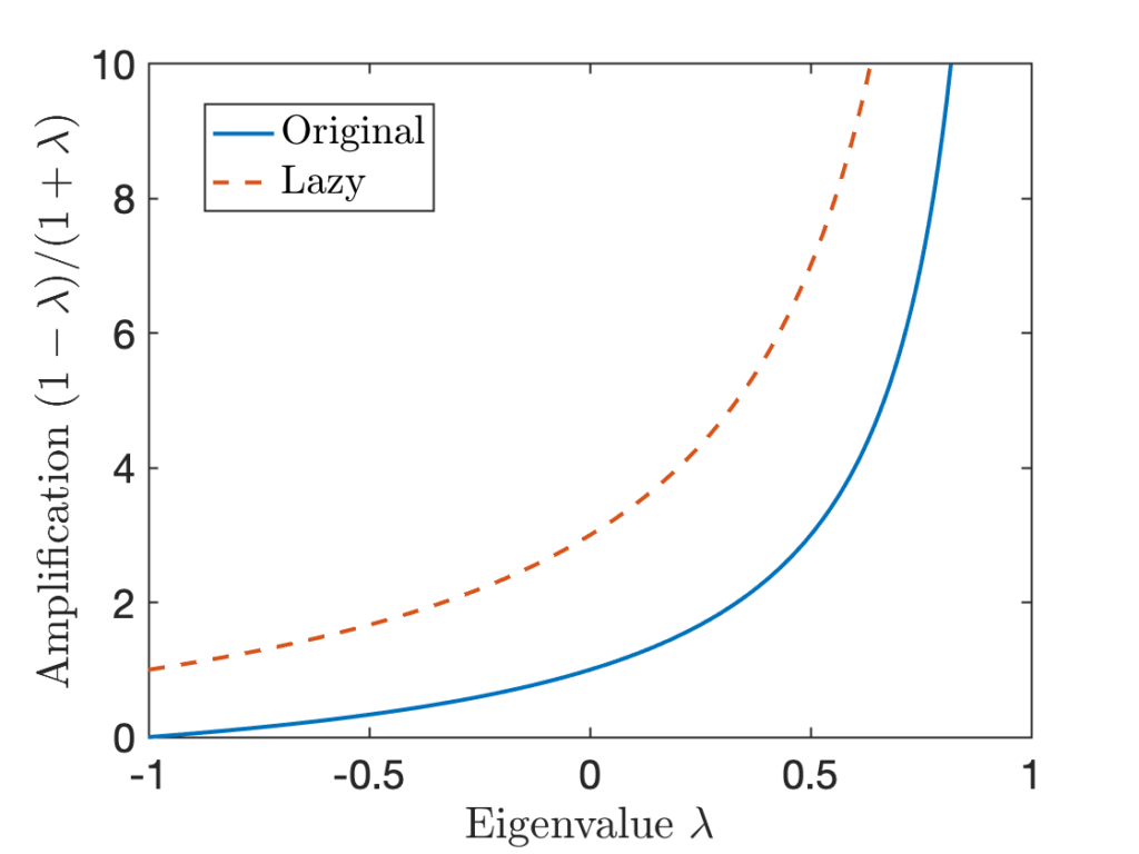
 with transition probability matrix
  and
and  and functions
  as being one and the same, and we will use both
  and
and  to denote the
  with a numeric value.
![\expect[f]](https://www.ethanepperly.com/wp-content/ql-cache/quicklatex.com-fb89f41552bdb76a7c8c04d9d35b3631_l3.png "Rendered by QuickLaTeX.com") denote the
denote the  where
where ![\[\expect[f] \coloneqq \expect_{X \sim \pi} [f(X)] = \sum_{i=1}^m \pi_i f(i).\]](https://www.ethanepperly.com/wp-content/ql-cache/quicklatex.com-09e6ff4df06017b52b788b6787fad904_l3.png "Rendered by QuickLaTeX.com")
![\[\Var(f) \coloneqq \expect [(f - \expect[f])^2] = \sum_{i=1}^m (f(i) - \expect[f])^2 \pi_i.\]](https://www.ethanepperly.com/wp-content/ql-cache/quicklatex.com-03395d1f27b782837abde9a7d030c4c7_l3.png "Rendered by QuickLaTeX.com")
 denote a probability distribution which assigns 100% probability to outcome
  matrix with real entries
  ) has
) has  .
. . Let’s first ask: What does the transpose
  is equipped with the
  and it is defined as
![\[(f,g) \coloneqq f^\top g = \sum_{i=1}^m f(i) g(i).\]](https://www.ethanepperly.com/wp-content/ql-cache/quicklatex.com-86465508e63dc4f1aefde253dd2b2a7c_l3.png "Rendered by QuickLaTeX.com")
![\[(f,Ag) = (A^\top f, g)\quad \text{for every }f,g\in\real^m.\]](https://www.ethanepperly.com/wp-content/ql-cache/quicklatex.com-9bc76899fbef0450c0757d9d90e3722a_l3.png "Rendered by QuickLaTeX.com")
 is the same as the amount of
  in the direction of
 ![[\cdot,\cdot]](https://www.ethanepperly.com/wp-content/ql-cache/quicklatex.com-9f5a656d3836fd9f84831aee0283adc1_l3.png "Rendered by QuickLaTeX.com") be any inner product on
be any inner product on  such that
 ![\[[f,Ag]=[A^*f,g]\quad\text{for every }f,g\in\real^m.\]](https://www.ethanepperly.com/wp-content/ql-cache/quicklatex.com-fe7c2788bf80274e17adc7bef25f9701_l3.png "Rendered by QuickLaTeX.com")
 .
.![\[[u_i,u_j]=\begin{cases}1, & i=j, \\0,& i\ne j.\end{cases}\]](https://www.ethanepperly.com/wp-content/ql-cache/quicklatex.com-6485908bc8e69e0ad6fb16b826344f60_l3.png "Rendered by QuickLaTeX.com")
![\[\langle f, g \rangle \coloneqq \expect[f\cdot g] = \sum_{i=1}^m f(i)g(i) \pi_i.\]](https://www.ethanepperly.com/wp-content/ql-cache/quicklatex.com-a1d97adbf15c3c5bd85460e94161ee28_l3.png "Rendered by QuickLaTeX.com")
![\expect[f] = \expect[g] = 0](https://www.ethanepperly.com/wp-content/ql-cache/quicklatex.com-16f996fb8f734dee3bcc58dc1b6638b1_l3.png "Rendered by QuickLaTeX.com") ), it reports the
), it reports the  where
where  is drawn from
  :
:
![\[\pi_i P_{ij} = \pi_j P_{ji} \quad \text{for } i,j=1,2,\ldots,m\]](https://www.ethanepperly.com/wp-content/ql-cache/quicklatex.com-d24fd7216a2b9a2afc49c2f1ae9ea55c_l3.png "Rendered by QuickLaTeX.com")
![\[\langle f, Pg \rangle= \sum_{i,j=1}^m f(i) g(j) \pi_jP_{ji} = \sum_{j=1}^m \left( \sum_{i=1}^m f(i) P_{ij} \right) g(j) \pi_j = \langle Pf, g\rangle.\]](https://www.ethanepperly.com/wp-content/ql-cache/quicklatex.com-2e8d0788b8c0f3ee0e4602e817957cfa_l3.png "Rendered by QuickLaTeX.com")
 associated with eigenvectors
  which are orthonormal in the
 ![\[\langle\varphi_i,\varphi_j\rangle=\begin{cases}1, &i=j\\0,& i\ne j.\end{cases}\]](https://www.ethanepperly.com/wp-content/ql-cache/quicklatex.com-fd0e99bc2439329beccce1339db0aee9_l3.png "Rendered by QuickLaTeX.com")
 span all of
  elsewhere. Then, by the fundamental theorem of Markov chains,
  converges to
  for every
  ,
,  . Thus, since
  for every vector
  in magnitude.
 is a vector of all one’s.
 have magnitude
  .
. for every
  .
. and
and ![\[\norm{\sigma - \pi}_{\rm TV} = \max_{A \subseteq \{1,\ldots,m\}} |\sigma(A) - \pi(A)| = \frac{1}{2} \sum_{i=1}^m |\sigma_i - \pi_i|.\]](https://www.ethanepperly.com/wp-content/ql-cache/quicklatex.com-d369d587213cfe7bb579ea5d2d89d1f8_l3.png "Rendered by QuickLaTeX.com")

 and
and  of each outcome. Spectral theory plays more nicely with an “
 ” way of comparing probability distributions, which we develop now.
 . This provides a general way of figuring out which objects for finite state space Markov chains are row vectors and which are column vectors: Measures are row vectors whereas functions are column vectors.
 given by
![\[h(i) = \frac{d\sigma}{d\pi}(i) = \frac{\sigma_i}{\pi_i} \quad \text{for } i=1,2,\ldots,m.\]](https://www.ethanepperly.com/wp-content/ql-cache/quicklatex.com-cbffacfb7f8993bd3f61752e12035912_l3.png "Rendered by QuickLaTeX.com")
![\[\expect_{X \sim \sigma} [g(X)] = \expect_{Y \sim \pi}[g(Y)h(Y)] = \sum_{i=1}^m g(i)h(i) \pi_i. \]](https://www.ethanepperly.com/wp-content/ql-cache/quicklatex.com-b0bf11be5c7b4508cf0965a0c53426ab_l3.png "Rendered by QuickLaTeX.com")
 is a random variable with distribution
 ![\mathrm{Unif}[0,1]](https://www.ethanepperly.com/wp-content/ql-cache/quicklatex.com-0db92c7166ac7b273b85e4c488d226ea_l3.png "Rendered by QuickLaTeX.com") ) is a function
) is a function ![\[\expect_{X \sim \sigma} [g(X)] = \expect_{Y\sim \mathrm{Unif}[0,1]} [g(Y)h(Y)] = \int_0^1 g(x) h(x) \, dx.\]](https://www.ethanepperly.com/wp-content/ql-cache/quicklatex.com-c7f33161d65ad1fcb0f79f24b4f51a0f_l3.png "Rendered by QuickLaTeX.com")
 replaced with integrals
  .
.
![\[\chi^2(\sigma \mid\mid \pi) \coloneqq \Var \left(\frac{d\sigma}{d\pi} \right) = \expect \left[\left( \frac{d\sigma}{d\pi} - 1 \right)^2\right] = \expect \left[\left(\frac{d\sigma}{d\pi}\right)^2\right] - 1.\]](https://www.ethanepperly.com/wp-content/ql-cache/quicklatex.com-2521b63ae50f02fe6099c54dcc4e00a4_l3.png "Rendered by QuickLaTeX.com")
 , note that
![\[\expect\left[\frac{d\sigma}{d\pi}\right] = \sum_{i=1}^m \frac{d\sigma}{d\pi}(i) \pi_i = \sum_{i=1}^m \frac{\sigma_i}{\pi_i} \pi_i = \sum_{i=1}^m \sigma_i = 1. \]](https://www.ethanepperly.com/wp-content/ql-cache/quicklatex.com-6bcec4a11dcc43c0b01738d12e38d6e6_l3.png "Rendered by QuickLaTeX.com")
![\[\norm{\sigma - \pi}_{\rm TV} = \frac{1}{2} \expect \left[ \left| \frac{d\sigma}{d\pi} - 1 \right| \right].\]](https://www.ethanepperly.com/wp-content/ql-cache/quicklatex.com-4ab771f36e4aabcf1fcbe807729630b6_l3.png "Rendered by QuickLaTeX.com")
![\[\norm{\sigma - \pi}_{\rm TV} = \frac{1}{2} \expect \left[ \left| \frac{d\sigma}{d\pi} - 1 \right| \right] \le \frac{1}{2} \left(\expect \left[ \left( \frac{d\sigma}{d\pi} - 1 \right)^2 \right]\right)^{1/2} = \frac{1}{2} \sqrt{\chi^2(\sigma \mid\mid \pi)}. \]](https://www.ethanepperly.com/wp-content/ql-cache/quicklatex.com-4986b7434b84b79aff6f94df2ec4b4e8_l3.png "Rendered by QuickLaTeX.com")
 denote the distributions of the Markov chain at times
  . Then
 and
and  ,
, ![\[\chi^2(\delta_i \mid\mid \pi) \le \frac{1}{\pi_i}. \]](https://www.ethanepperly.com/wp-content/ql-cache/quicklatex.com-4896a0499c8c3b1ab5bc1e2952fd1d65_l3.png "Rendered by QuickLaTeX.com")
![\[\chi^2\left( \rho^{(0)} \, \middle|\middle| \, \pi \right) \le \frac{1}{\min_{1\le i\le m} \pi_i} \]](https://www.ethanepperly.com/wp-content/ql-cache/quicklatex.com-c3a7cb7312400b0230e1a53951e6d0a7_l3.png "Rendered by QuickLaTeX.com")
![\[\chi^2(\delta_i \mid\mid \pi) = \Var(d\delta_i/d\pi) \le \expect[(d\delta_i/d\pi)^2] = 1/\pi_i.\]](https://www.ethanepperly.com/wp-content/ql-cache/quicklatex.com-7343459c314bf5425643e99e6f0e2906_l3.png "Rendered by QuickLaTeX.com")
 is a
is a  for some
 ![\[\norm{\rho^{(n)} - \pi}_{\rm TV} \le \varepsilon\]](https://www.ethanepperly.com/wp-content/ql-cache/quicklatex.com-5ed1f6d26bba1fa54f9bd01bcf39defc_l3.png "Rendered by QuickLaTeX.com")
![\[n = \left\lceil \frac{1}{\log(\max\{\lambda_2,-\lambda_n\})}\log \left( \frac{1}{2\varepsilon \min_{1\le i \le m}\sqrt{\pi_i}} \right) \right\rceil \text{ steps}. \]](https://www.ethanepperly.com/wp-content/ql-cache/quicklatex.com-8d9dc3295020a8171795dec7e448eef5_l3.png "Rendered by QuickLaTeX.com")

 . To do this, we use the recurrence for the probability distribution:
![\[\rho^{(n+1)}_j = \sum_{i=1}^m \rho_i^{(n)} P_{ij}.\]](https://www.ethanepperly.com/wp-content/ql-cache/quicklatex.com-84dcc77d0a4138d7d59160bcf259be32_l3.png "Rendered by QuickLaTeX.com")
![\[\left( \frac{d\rho^{(n+1)}}{d\pi}\right)_j = \frac{\rho_j^{(n+1)}}{\pi_j} = \frac{\sum_{i=1}^m \rho^{(n)}_i P_{ij}}{\pi_j}= \sum_{i=1}^m \rho^{(n)}_i\frac{P_{ij}}{\pi_j}.\]](https://www.ethanepperly.com/wp-content/ql-cache/quicklatex.com-b6c60937b23d2509e4a3e4fa1f121427_l3.png "Rendered by QuickLaTeX.com")
 , which implies
![\[\left( \frac{d\rho^{(n+1)}}{d\pi}\right)_j = \sum_{i=1}^m\rho^{(n)}_i \frac{P_{ji}}{\pi_i} = \sum_{i=1}^m P_{ji} \frac{\rho^{(n)}_i}{\pi_i} = \left( P \frac{d \rho^{(n)}}{d\pi} \right)_j.\]](https://www.ethanepperly.com/wp-content/ql-cache/quicklatex.com-d22315b80e3fc4d3736d0c49f877fa9c_l3.png "Rendered by QuickLaTeX.com")
 is an ordinary
 ![\[\frac{d\rho^{(n+1)}}{d\pi} = P \frac{d\rho^{(n)}}{d\pi} \quad \text{for } n =0,1,\ldots. \]](https://www.ethanepperly.com/wp-content/ql-cache/quicklatex.com-406471ab024dae5551eae8b499a0243e_l3.png "Rendered by QuickLaTeX.com")
![\[\frac{d\rho^{(0)}}{d\pi} = c_1 \mathbf{1} + c_2 \varphi_2 + \cdots + c_m \varphi_m.\]](https://www.ethanepperly.com/wp-content/ql-cache/quicklatex.com-6bcb8bbdd130a3e85c422adc2f37715d_l3.png "Rendered by QuickLaTeX.com")
![\expect[d\rho^{(0)}/d\pi] = 1](https://www.ethanepperly.com/wp-content/ql-cache/quicklatex.com-37f5774410e7d60045c0758953e0cdde_l3.png "Rendered by QuickLaTeX.com") . Thus, we conclude
. Thus, we conclude  . Since the
  are eigenvectors of
  , the recurrence (7) implies
![\[\frac{d\rho^{(n)}}{d\pi} = \mathbf{1} + c_2 \lambda_2^n \varphi_2 + \cdots + c_m \lambda_m^n \varphi_m.\]](https://www.ethanepperly.com/wp-content/ql-cache/quicklatex.com-935cf156fcf1f467b0c6719614b94e6b_l3.png "Rendered by QuickLaTeX.com")
![\[\chi^2(\rho^{(n)} \mid\mid \pi) = \sum_{i=2}^m c_i^2 \lambda_i^{2n} \le (\max \{ \lambda_2, -\lambda_m \})^{2n} \sum_{i=2}^m c_i^2 = (\max \{ \lambda_2, -\lambda_m \})^{2n} \chi^2(\rho^{(0)} \mid\mid \pi).\]](https://www.ethanepperly.com/wp-content/ql-cache/quicklatex.com-7b82e2d3cefcede8d4a7a72b1fa3ceea_l3.png "Rendered by QuickLaTeX.com")
![\[\tau_{\rm mix} \coloneqq \min \left\{ n \ge 1 : \max_{\rho^{(0)}} \norm{\rho^{(n)} - \pi}_{\rm TV} \le \frac{1}{2e} \right\}.\]](https://www.ethanepperly.com/wp-content/ql-cache/quicklatex.com-e491d914ce283944ca10dc9d96bdb1a5_l3.png "Rendered by QuickLaTeX.com")
 of the chain at time
  is the
 ![\[\norm{\rho^{(n)} - \pi}_{\rm TV} \le e^{-\lfloor n / \tau_{\rm mix}\rfloor}.\]](https://www.ethanepperly.com/wp-content/ql-cache/quicklatex.com-8a28da28e02550f209ce8ec1c8b5b79e_l3.png "Rendered by QuickLaTeX.com")
 , then
  .
. .
. such that (A) each process is individually a Markov chain with transition matrix
 ![\[\prob\{x_{n+1} = j \mid x_n = i \} = \prob\{y_{n+1} = j \mid y_n = i \} = P_{ij}\]](https://www.ethanepperly.com/wp-content/ql-cache/quicklatex.com-8a91e29baa6fd219723bc325c68d9b75_l3.png "Rendered by QuickLaTeX.com")
 , then
  .
. and
and  is initialized in the stationary distribution
  . Let
. Let  be the time at which
 ![\[\tau_{\rho^{(0)}} \coloneqq \min\{ n \ge 0 : x_n = y_n\}.\]](https://www.ethanepperly.com/wp-content/ql-cache/quicklatex.com-68580815d8347111c8a35c6767c24d3e_l3.png "Rendered by QuickLaTeX.com")
 control the convergence of the Markov chain
  .
.![\tau_{\rm mix} \le 2e \max_{\rho^{(0)}} \expect[\tau_{\rho^{(0)}}]](https://www.ethanepperly.com/wp-content/ql-cache/quicklatex.com-6bff20b3e6944c95a1e8bf2d625c22d0_l3.png "Rendered by QuickLaTeX.com") .
.![\[\norm{\rho^{(n)} - \pi}_{\rm TV} \le \prob\{\tau_{\rho^{(0)}} > n\}\le \frac{\expect[\tau_{\rho^{(0)}}]}{n}.\]](https://www.ethanepperly.com/wp-content/ql-cache/quicklatex.com-74fd53f9c863d5faf2edb9698e58854f_l3.png "Rendered by QuickLaTeX.com")
 . Then the left-hand side is at most
  , so
, so![\[\frac{1}{2e} \le \max_{\rho^{(0)}}\norm{\rho^{(\tau_{\rm mix})} - \pi}_{\rm TV} = \prob\{\tau_{\rho^{(0)}} > n\} \le \frac{\max_{\rho^{(0)}}\expect[\tau_{\rho^{(0)}}]}{\tau_{\rm mix}}.\]](https://www.ethanepperly.com/wp-content/ql-cache/quicklatex.com-61cf831f4db72e776d3122e3e323b7c1_l3.png "Rendered by QuickLaTeX.com")
 ). Therefore, one can also think of this Markov chain as a very inefficient way of generating a string of random bits.
 and a (uniform) random bit
  . Set
. Set  by changing the
  th bit of
  , and set
  by changing the
  to
to  have been chosen by time
  to be the time at which all positions
 ![\[\tau_{\rho^{(0)}} \le \tau_{\rm pick}.\]](https://www.ethanepperly.com/wp-content/ql-cache/quicklatex.com-878ab3b502681c3fb7c0453599af3293_l3.png "Rendered by QuickLaTeX.com")
![\expect[\tau_{\rm pick}]](https://www.ethanepperly.com/wp-content/ql-cache/quicklatex.com-ff405a11db183f95baecf7299661c685_l3.png "Rendered by QuickLaTeX.com") , it can be helpful to break into easier pieces. Let’s start with the simplest possible question: How many picks do we need to collect the first coupon? Just one. We always get a coupon in our first box.
, it can be helpful to break into easier pieces. Let’s start with the simplest possible question: How many picks do we need to collect the first coupon? Just one. We always get a coupon in our first box. of them are different from the first. So the probability of picking a new coupon in the second box is
  . In fact,
 , and its mean is
  . On average, we need
  picks to collect the second coupon.
 coupons we haven’t collected and
  . Thus, the number of picks is a geometric random variable with success probability
  .
. picks to pick the
  , we obtain that the total number of picks required is to collect all the coupons is
![\[\expect[\tau_{\rm pick}] = 1 + \frac{N}{N-1} + \frac{N}{N-2} + \cdots + \frac{N}{N-(N-1)} = N \left( \frac{1}{N} + \frac{1}{N-1} + \cdots + \frac{1}{2} + 1 \right).\]](https://www.ethanepperly.com/wp-content/ql-cache/quicklatex.com-db166dbcfe9198024b7dafb5de81fdf7_l3.png "Rendered by QuickLaTeX.com")
 denote the
 ![\[H_N = 1 + \frac{1}{2} + \cdots + \frac{1}{N}\]](https://www.ethanepperly.com/wp-content/ql-cache/quicklatex.com-280c58a265450ae987b6c6236999bfd0_l3.png "Rendered by QuickLaTeX.com")
![\expect[\tau_{\rm pick}] = NH_N](https://www.ethanepperly.com/wp-content/ql-cache/quicklatex.com-ec1cac0ce484b5e1ceef29a198523670_l3.png "Rendered by QuickLaTeX.com") . Since the
. Since the  , we have
![\[\expect[\tau_{\rm pick}] \le N \log (N) + N.\]](https://www.ethanepperly.com/wp-content/ql-cache/quicklatex.com-2626a01a852627593ced1766177dcbbc_l3.png "Rendered by QuickLaTeX.com")
![\[\tau_{\rm mix} \le 2e \, \expect[\tau_{\rho^{(0)}}] \le 2e \, \expect[\tau_{\rm pick}] \le 2e \, N \log(N) + 2e \, N.\]](https://www.ethanepperly.com/wp-content/ql-cache/quicklatex.com-73215e6c39a6bd7162aba749cd61e1bf_l3.png "Rendered by QuickLaTeX.com")
 .
.
![\[\prob\{\tau_{\rm pick} > N \log N + cN\} \le e^{-c}\]](https://www.ethanepperly.com/wp-content/ql-cache/quicklatex.com-73f8883bcb323760364995473bcc3831_l3.png "Rendered by QuickLaTeX.com")
 and
and  , from which it follows that
![\[\norm{\rho^{(n)} - \pi}_{\rm TV} \le \varepsilon \quad \text{provided that} \quad n \ge N \log N + N \log(1/\varepsilon).\]](https://www.ethanepperly.com/wp-content/ql-cache/quicklatex.com-14c0bb8d63f118fc70a87253f64236af_l3.png "Rendered by QuickLaTeX.com")
![\[\norm{\rho^{(n)} - \pi}_{\rm TV} \le \varepsilon \quad \text{provided that} \quad n \ge \frac{1}{2} N \log N + c \,N \log(1/\varepsilon)\]](https://www.ethanepperly.com/wp-content/ql-cache/quicklatex.com-ce2a7b130eee9537cf737b90814aa4d3_l3.png "Rendered by QuickLaTeX.com")
 . The constant
  in this inequality cannot be improved. See section 5.3.1 of
  . When initialized from any starting distribution
  if all of its entries are strictly positive. Recall that a Markov chain with transition matrix
  . For this post, all Markov chains will have state space
  and
and ![\[\norm{\rho - \sigma}_{\rm TV} = \max_{S \subseteq \{1,\ldots,m\}} |\rho(S) - \sigma(S)| = \frac{1}{2} \sum_{i=1}^m \left| \rho_i - \sigma_i \right|.\]](https://www.ethanepperly.com/wp-content/ql-cache/quicklatex.com-7dd0b0e121d45408883369794becedff_l3.png "Rendered by QuickLaTeX.com")
 .
. . Thus, despite these distributions seeming quite similar to us, the total variation distance between
  , if
, if![\[\prob \{x = i\} = \rho_i \quad \text{for $i=1,2,\ldots,m$}.\]](https://www.ethanepperly.com/wp-content/ql-cache/quicklatex.com-3537663be586f21278e7e32b7502af94_l3.png "Rendered by QuickLaTeX.com")
 on
on  is a distribution on
  such that if a pair of random variables
  is drawn from
  . Denote the set of all couplings of
  .
.![\[\norm{\rho - \sigma}_{\rm TV} = \min_{\gamma \in \operatorname{Couplings}(\rho,\sigma)} \prob_{(x,y) \sim \gamma} \{ x \ne y \}.\]](https://www.ethanepperly.com/wp-content/ql-cache/quicklatex.com-918278c5556c178aee214db808000551_l3.png "Rendered by QuickLaTeX.com")
 represents the probability for variables
  drawn from joint distribution
  . Then the coupling lemma tells us that there is a coupling
  . Indeed, such a coupling can be obtained by drawing
  . This defines a joint distribution
  with 100% probability.
 ,
, ![\[\norm{\rho - \sigma}_{\rm TV} \le \prob \{x \ne y \}.\]](https://www.ethanepperly.com/wp-content/ql-cache/quicklatex.com-2b881043ba005f53ae84ada8ebe53191_l3.png "Rendered by QuickLaTeX.com")
![\[\norm{\rho - \sigma}_{\rm TV} = \prob \{x \ne y\}.\]](https://www.ethanepperly.com/wp-content/ql-cache/quicklatex.com-e692d3e9715ed9b325be70775ba0eac3_l3.png "Rendered by QuickLaTeX.com")
 as
as  at an exponential rate.
 is non-increasing
 ![\[\norm{\rho^{(n+1)} - \pi}_{\rm TV} \le \norm{\rho^{(n)} - \pi}_{\rm TV} \quad \text{for every } n =0,1,2\ldots. \]](https://www.ethanepperly.com/wp-content/ql-cache/quicklatex.com-49f8b3e1681a778cc0540ab25def9d1c_l3.png "Rendered by QuickLaTeX.com")
![\[\norm{\rho^{(n)} - \pi}_{\rm TV} = \prob \{x_n\ne y_n\}.\]](https://www.ethanepperly.com/wp-content/ql-cache/quicklatex.com-8e78bf69e3ca31ba02e37fa3a64e5f52_l3.png "Rendered by QuickLaTeX.com")
 .
. , then run the two chains
 ![\[\prob\{x_{n+1}\ne y_{n+1}\} \le \prob\{x_n \ne y_n\}.\]](https://www.ethanepperly.com/wp-content/ql-cache/quicklatex.com-3904173ffb700f39526fb117f5a6c248_l3.png "Rendered by QuickLaTeX.com")
![\[\norm{\rho^{(n+1)} - \pi}_{\rm TV} \le \prob\{x_{n+1}\ne y_{n+1}\} \le \prob\{x_n \ne y_n\} = \norm{\rho^{(n)} - \pi}_{\rm TV}.\]](https://www.ethanepperly.com/wp-content/ql-cache/quicklatex.com-2409e83e870c68fe8d7f8e1a94903325_l3.png "Rendered by QuickLaTeX.com")
 .
. more carefully. Write it as
 , break into cases for all possible values
  for
for  to take
 be the minimum probability of moving between any two states
![\[p_{\rm min} \coloneqq \min_{1\le i,j\le m} P_{ij}.\]](https://www.ethanepperly.com/wp-content/ql-cache/quicklatex.com-ca934d28f674adb9b8bc14ef320dd327_l3.png "Rendered by QuickLaTeX.com")
 to
to 
![\[\prob \{x_{n+1} \ne y_{n+1}\} \le (1 - p_{\rm min})\prob \{x_n \ne y_n\}.\]](https://www.ethanepperly.com/wp-content/ql-cache/quicklatex.com-69b8b6e06ad981139c7c6ffd1ae6d1ba_l3.png "Rendered by QuickLaTeX.com")
![\[\norm{\rho^{(n+1)}-\pi}_{\rm TV} \le \prob \{x_{n+1} \ne y_{n+1}\} \le (1 - p_{\rm min})\prob \{x_n \ne y_n\} = (1 - p_{\rm min}) \norm{\rho^{(n)} - \pi}_{\rm TV}.\]](https://www.ethanepperly.com/wp-content/ql-cache/quicklatex.com-ce7570327a59ec2ede1a579d7f13564d_l3.png "Rendered by QuickLaTeX.com")
![\[\norm{\rho^{(n)} - \pi}_{\rm TV} \le (1 - p_{\rm min})^n \norm{\rho^{(0)} - \pi}_{\rm TV} \le (1 - p_{\rm min})^n.\]](https://www.ethanepperly.com/wp-content/ql-cache/quicklatex.com-9119337225ce34aa99582b2b53069300_l3.png "Rendered by QuickLaTeX.com")
 . Fortunately, together with our earlier observation that distance to stationarity is non-increasing, we can upgrade this proof into a proof for the general case.
 for which
  . Construct an auxilliary Markov chain
  such that one step of the auxilliary chain consists of running
 ![\[z_0 = x_0, \:z_1 = x_{n_0}, \:z_2 = x_{2n_0},\ldots.\]](https://www.ethanepperly.com/wp-content/ql-cache/quicklatex.com-e5c67b34610d3cf8834e42621fd85218_l3.png "Rendered by QuickLaTeX.com")
 is
is  , we have
![\[\norm{\rho^{(k\cdot n_0)} - \pi}_{\rm TV} \le (1-\delta)^k \norm{\rho^{(0)} - \pi}_{\rm TV} \le (1-\delta)^k \quad \text{for }k=0,1,2,\ldots,\]](https://www.ethanepperly.com/wp-content/ql-cache/quicklatex.com-f00ec64a989f2c387244cc13ca79cb63_l3.png "Rendered by QuickLaTeX.com")
 . Thus, since distance to stationarity is non-increasing, we have
![\[\norm{\rho^{(n)} - \pi}_{\rm TV} \le \norm{\rho^{(n_0 \cdot \lfloor n/n_0\rfloor)} - \pi}_{\rm TV} \le (1-\delta)^{\lfloor n/n_0\rfloor} \norm{\rho^{(0)} - \pi}_{\rm TV} \le (1-\delta)^{\lfloor n/n_0\rfloor}.\]](https://www.ethanepperly.com/wp-content/ql-cache/quicklatex.com-c8c82df8e81ce5b1ca4fcbae23a11f4d_l3.png "Rendered by QuickLaTeX.com")
![\[\tau_{\rm mix} \coloneqq \min \left\{ n \ge 1 : \max_{\rho^{(0)}} \norm{\rho^{(n)} - \pi}_{\rm TV} \le \frac{1}{2e} \right\}.\]](https://www.ethanepperly.com/wp-content/ql-cache/quicklatex.com-ccf82253d6d08b59e651ef0c81a44e57_l3.png "Rendered by QuickLaTeX.com")
 steps:
 , then
  be the expected number of times the chain hits
  . Because the chain is primitive, all of the
 ![\[\pi_i = \frac{a_i}{\sum_{j=1}^m a_j}.\]](https://www.ethanepperly.com/wp-content/ql-cache/quicklatex.com-6abd189895ccf9707e3178558a0b5a2c_l3.png "Rendered by QuickLaTeX.com")
![\[a^\top P = a^\top. \]](https://www.ethanepperly.com/wp-content/ql-cache/quicklatex.com-d6885d4de71a8b8655bd542c1434c775_l3.png "Rendered by QuickLaTeX.com")
 denote the values of the chain and
  denote the time at which the chain returns to
 ![\[a_j = \sum_{n=1}^\infty \prob\{x_n = j, n_{\rm ret} > n\}.\]](https://www.ethanepperly.com/wp-content/ql-cache/quicklatex.com-713cac4a8c97033b1cba87fe2632d46d_l3.png "Rendered by QuickLaTeX.com")
![\[a_j = \prob\{x_1 = j\} + \sum_{n=2}^\infty \prob\{x_n = j, n_{\rm ret} > n\}.\]](https://www.ethanepperly.com/wp-content/ql-cache/quicklatex.com-1f62dfb50726f4884c2cb790970d1a75_l3.png "Rendered by QuickLaTeX.com")
 . For the second term, break into cases depending on the value of the chain at time
![\[a_j = P_{ij} + \sum_{n=2}^\infty \sum_{k\ne i} \prob\{x_{n-1} = k, n_{\rm ret} > n-1 \} P_{kj}.\]](https://www.ethanepperly.com/wp-content/ql-cache/quicklatex.com-f243b52714b96a419b94980a12f078ee_l3.png "Rendered by QuickLaTeX.com")
 to
to  and exchange the order of summation to obtain
![\[a_j = P_{ij} + \sum_{k\ne i} \left(\sum_{n=1}^\infty \prob\{x_n = k, n_{\rm ret} > n \}\right) P_{kj}.\]](https://www.ethanepperly.com/wp-content/ql-cache/quicklatex.com-cad1677f621e66a91f850ab352cedce0_l3.png "Rendered by QuickLaTeX.com")
 . Thus, since
  , we have
![\[a_j = a_iP_{ij} + \sum_{k\ne i} a_k P_{kj} = \sum_{k=1}^m a_k P_{kj},\]](https://www.ethanepperly.com/wp-content/ql-cache/quicklatex.com-cecaa5c06b9ce9d9c3f4aa814dfc2323_l3.png "Rendered by QuickLaTeX.com")
 be a matrix and
  measured in some
  ? How do these answers change with different norms?
 get except for some small failure probability
  ?
?![\[\mathbb{E} \left\|B-X\right\|_{\rm F}^2 \le \left( 1 + \frac{k}{k-(r+1)}\right) \left\|B - \lowrank{B}_r \right\|_{\rm F}^2 \quad \text{for every $r \le k-2$}.\]](https://www.ethanepperly.com/wp-content/ql-cache/quicklatex.com-6759ab11982f765f19dc615fb8e1fbdc_l3.png "Rendered by QuickLaTeX.com")
 is the
  where
where  , where
  denotes the
 ![\[B\approx X \coloneqq QC.\]](https://www.ethanepperly.com/wp-content/ql-cache/quicklatex.com-dbf0ef5be3e2a7fc39d609f4621d2dbd_l3.png "Rendered by QuickLaTeX.com")
 into a
  , as we did as steps 4 and 5 in the previous post.
![\[X = QC = QQ^*B = \Pi_{B\Omega} B.\]](https://www.ethanepperly.com/wp-content/ql-cache/quicklatex.com-0d1ae78fbe7d6d4d91b567795bd91f57_l3.png "Rendered by QuickLaTeX.com")
 denotes the
  . We call
  the projection formula for the randomized SVD.
 is
is ![\[U^*U = UU^* = I.\]](https://www.ethanepperly.com/wp-content/ql-cache/quicklatex.com-33fedf7ef9e12832ea6188011e3874bd_l3.png "Rendered by QuickLaTeX.com")
 on matrices is
 ![\[\left\|UBV\right\|_{\rm UI} = \left\|B\right\|_{\rm UI} \quad \text{for all unitary matrices $U$, $V$ and any matrix $B$}.\]](https://www.ethanepperly.com/wp-content/ql-cache/quicklatex.com-5fd16f43277f7e25ee2f910665984e09_l3.png "Rendered by QuickLaTeX.com")
 is said to be quadratic if there exists another unitarily invariant norm
 ![\[\left\|B\right\|_{\rm Q}^2 = \left\|B^*B\right\|_{\rm UI} = \left\|BB^*\right\|_{\rm UI} \quad \text{for every matrix $B$.} \]](https://www.ethanepperly.com/wp-content/ql-cache/quicklatex.com-aac3c6aec691fb438adf6690682d855d_l3.png "Rendered by QuickLaTeX.com")
![\[\left\|B\right\|_{S_p}^p \coloneqq \sum_i \sigma_i(B)^p.\]](https://www.ethanepperly.com/wp-content/ql-cache/quicklatex.com-d032386a33d5df74c8a44235dafac359_l3.png "Rendered by QuickLaTeX.com")
 denote the decreasingly order
  -norm
-norm  is the
 ![\[\norm{B} = \left\|B\right\|_{S_\infty} \coloneqq \max_i \sigma_i(B) = \sigma_1(B).\]](https://www.ethanepperly.com/wp-content/ql-cache/quicklatex.com-584051e6c083d9b865ffe52d79186a00_l3.png "Rendered by QuickLaTeX.com")
 . However, the Schatten
  since
since![\[\left\|B\right\|_{S_p}^2 = \left\|B^*B\right\|_{S_{p/2}}.\]](https://www.ethanepperly.com/wp-content/ql-cache/quicklatex.com-27e888ecff0b0c38df6e73a803f8aa1d_l3.png "Rendered by QuickLaTeX.com")
![\[\left\|B - X\right\|_{\rm Q}^2 \le \left\|B - \lowrank{B}_r\right\|_{\rm Q}^2 + \left\|\lowrank{B}_r - \Pi_{B\Omega} \lowrank{B}_r\right\|_{\rm Q}^2. \]](https://www.ethanepperly.com/wp-content/ql-cache/quicklatex.com-c1738a10a5c46d5455b8e2d5992ce98d_l3.png "Rendered by QuickLaTeX.com")
 to be an optimal rank-
 approximation to
 ![\[\left\|B - \lowrank{B\right\|_r}_{\rm Q} \le \left\|B - C\right\|_{\rm Q} \quad \text{for any rank-$r$ matrix $C$}.\]](https://www.ethanepperly.com/wp-content/ql-cache/quicklatex.com-46106e1ebeaa349721ea4e81d171f70b_l3.png "Rendered by QuickLaTeX.com")
![\[\left\|B - X\right\|_{\rm Q}^2 - \left\|B - \lowrank{B}_r\right\|_{\rm Q}^2 \le \left\|\lowrank{B}_r - \Pi_{B\Omega} \lowrank{B}_r\right\|_{\rm Q}^2.\]](https://www.ethanepperly.com/wp-content/ql-cache/quicklatex.com-e44e6de74ec072bf3d6c944ea6de77db_l3.png "Rendered by QuickLaTeX.com")

 and
and  , and the third is the triangle inequality. For the fifth line, we use the fact that
  is an orthoprojector and thus has unit spectral norm
  together with the fact that
![\[\left\|BCD\right\|_{\rm UI} \le \norm{B} \cdot \left\|C\right\|_{\rm UI}\cdot \norm{D} \quad \text{for all matrices $B,C,D$.}\]](https://www.ethanepperly.com/wp-content/ql-cache/quicklatex.com-e329f332e4305af288668bfdf1ab4bf5_l3.png "Rendered by QuickLaTeX.com")
![\[(B - \lowrank{B}_r)(B - \lowrank{B}_r)^* = BB^* - \lowrank{B}_r\lowrank{B}_r^*.\]](https://www.ethanepperly.com/wp-content/ql-cache/quicklatex.com-9db3f7e6eb57261b556783a0a7d62fd0_l3.png "Rendered by QuickLaTeX.com")
![\[B = \onebytwo{U_1}{U_2} \twobytwo{\Sigma_1}{0}{0}{\Sigma_2}\onebytwo{V_1}{V_2}^*\]](https://www.ethanepperly.com/wp-content/ql-cache/quicklatex.com-54a749c18b5a76a0f468adee8b5fa58f_l3.png "Rendered by QuickLaTeX.com")
 and
and  both have orthonormal columns,
 and
and  are square diagonal matrices with nonnegative entries,
 and
and  have
have  matrix.
 . Define
![\[\twobyone{\Omega_1}{\Omega_2} \coloneqq \twobyone{V_1^*}{V_2^*} \Omega.\]](https://www.ethanepperly.com/wp-content/ql-cache/quicklatex.com-f620ec79bd8a3f6022efb5ca07b0d824_l3.png "Rendered by QuickLaTeX.com")
 is full-rank (i.e.,
  ).
).
 so
so![\[\norm{(I-\Pi_{B\Omega})U_1\Sigma_1}_{\rm Q}^2 \le \norm{(I-\Pi_{B\Omega\Omega_1^\dagger})U_1\Sigma_1}_{\rm Q}^2 = \norm{\Sigma_1U_1^*(I-\Pi_{B\Omega\Omega_1^\dagger})U_1\Sigma_1}_{\rm UI}. \]](https://www.ethanepperly.com/wp-content/ql-cache/quicklatex.com-2fdd85edd3e561ae5496031960d8901a_l3.png "Rendered by QuickLaTeX.com")
![\[\Sigma_1U_1^*(I-\Pi_{B\Omega\Omega_1^\dagger})U_1\Sigma_1.\]](https://www.ethanepperly.com/wp-content/ql-cache/quicklatex.com-f21f88902abb8532d54b098fa358ddc0_l3.png "Rendered by QuickLaTeX.com")
![\[B\Omega\Omega_1^\dagger = B\onebytwo{V_1}{V_2}\twobyone{\Omega_1}{\Omega_2}\Omega_1^\dagger = \onebytwo{U_1}{U_2} \twobytwo{\Sigma_1}{0}{0}{\Sigma_2} \twobyone{I}{\Omega_2\Omega_1^\dagger} = U_1\Sigma_1 + U_2\Sigma_2\Omega_2\Omega_1^\dagger.\]](https://www.ethanepperly.com/wp-content/ql-cache/quicklatex.com-e1dbcff75c12101b6274492896899b52_l3.png "Rendered by QuickLaTeX.com")
 takes the form
![\begin{align*}\Pi_{B\Omega\Omega_1^\dagger} &= (B\Omega\Omega_1^\dagger) \left[(B\Omega\Omega_1^\dagger)^*(B\Omega\Omega_1^\dagger)\right]^\dagger (B\Omega\Omega_1^\dagger)^* \\&= (U_1\Sigma_1 + U_2\Sigma_2\Omega_2\Omega_1^\dagger) \left[\Sigma_1^2 + (\Sigma_2\Omega_2\Omega_1^\dagger)^*(\Sigma_2\Omega_2\Omega_1^\dagger)\right]^\dagger (U_1\Sigma_1 + U_2\Sigma_2\Omega_2\Omega_1^\dagger)^*.\end{align*}](https://www.ethanepperly.com/wp-content/ql-cache/quicklatex.com-d9e0cd585357787c460f6471f52ecb0a_l3.png "Rendered by QuickLaTeX.com")
 denotes the
 ![\[\Sigma_1U_1^*(I-\Pi_{B\Omega\Omega_1^\dagger})U_1\Sigma_1 = \Sigma_1^2 - \Sigma_1^2 \left[\Sigma_1^2 + (\Sigma_2\Omega_2\Omega_1^\dagger)^*(\Sigma_2\Omega_2\Omega_1^\dagger)\right]^\dagger\Sigma_1^2. \]](https://www.ethanepperly.com/wp-content/ql-cache/quicklatex.com-b7dfa3f3cbcda5380b6b7ec0132fca2a_l3.png "Rendered by QuickLaTeX.com")
 is defined as
![\[A : H \coloneqq A - A(A+H)^\dagger A. \]](https://www.ethanepperly.com/wp-content/ql-cache/quicklatex.com-0ca6dd2810aa560e0d59d808c9b40bc8_l3.png "Rendered by QuickLaTeX.com")
![\[\Sigma_1U_1^*(I-\Pi_{B\Omega\Omega_1^\dagger})U_1\Sigma_1 = \Sigma_1^2 : [(\Sigma_2\Omega_2\Omega_1^\dagger)^*(\Sigma_2\Omega_2\Omega_1^\dagger)].\]](https://www.ethanepperly.com/wp-content/ql-cache/quicklatex.com-dc620e38c4fb8a7855e330183c8313c9_l3.png "Rendered by QuickLaTeX.com")
![\[\left\|B - X\right\|_{\rm Q}^2\le \left\| \Sigma_2 \right\|_{\rm Q}^2 + \left\|\Sigma_1^2 : [(\Sigma_2\Omega_2\Omega_1^\dagger)^*(\Sigma_2\Omega_2\Omega_1^\dagger)]\right\|_{\rm UI}. \]](https://www.ethanepperly.com/wp-content/ql-cache/quicklatex.com-ff8a161c38344c97e0d615d216d4555d_l3.png "Rendered by QuickLaTeX.com")
 . The
. The  is given by
 ![\[v = a \cdot \mathrm{curr}_a.\]](https://www.ethanepperly.com/wp-content/ql-cache/quicklatex.com-50ff6a1f099e535f6dfd8525f45b4741_l3.png "Rendered by QuickLaTeX.com")
 is then
![\[v = h \cdot \mathrm{curr}_h.\]](https://www.ethanepperly.com/wp-content/ql-cache/quicklatex.com-baea64abba5be2425a04d7d2316f7153_l3.png "Rendered by QuickLaTeX.com")
![\[\mathrm{curr}_{\rm total} = \mathrm{curr}_a + \mathrm{curr}_h = \frac{v}{a} + \frac{v}{h} = v \left(a^{-1}+h^{-1}\right).\]](https://www.ethanepperly.com/wp-content/ql-cache/quicklatex.com-2ce6cd66280641977f8eea4d3d9f6cab_l3.png "Rendered by QuickLaTeX.com")
![\[a:h \coloneqq \frac{v}{\mathrm{curr}_{\rm total}} = \left( a^{-1}+h^{-1}\right)^{-1}. \]](https://www.ethanepperly.com/wp-content/ql-cache/quicklatex.com-46eba66bdf328c974e763d8c43422e75_l3.png "Rendered by QuickLaTeX.com")
 the parallel sum of
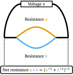
 can be extended to all nonnegative numbers
 ![\[a:h \coloneqq \lim_{b\downarrow a, \: k\downarrow h} b:k = \begin{cases}\left( a^{-1}+h^{-1}\right)^{-1}, & a,h > 0 ,\\0, & \textrm{otherwise}.\end{cases}\]](https://www.ethanepperly.com/wp-content/ql-cache/quicklatex.com-7c49cbcbcd8d8f75fa4f18a40562e718_l3.png "Rendered by QuickLaTeX.com")
![\[A:H = (A^{-1}+H^{-1})^{-1} \quad \text{for $A,H$ positive definite.}\]](https://www.ethanepperly.com/wp-content/ql-cache/quicklatex.com-95cd7707ba37e3436926c73895d537bb_l3.png "Rendered by QuickLaTeX.com")
![\[a:h = \frac{1}{a^{-1}+h^{-1}} = \frac{ah}{a+h} = \frac{a(a+h)-a^2}{a+h} = a - a(a+h)^{-1}a.\]](https://www.ethanepperly.com/wp-content/ql-cache/quicklatex.com-e4e355840ccdeb857cec59c1173cca5b_l3.png "Rendered by QuickLaTeX.com")
![\[A : H = A - A(A+H)^\dagger A.\]](https://www.ethanepperly.com/wp-content/ql-cache/quicklatex.com-85f7337339efbd593339ed3a5ff7e547_l3.png "Rendered by QuickLaTeX.com")
 ,
, for positive definite matrices,
 and
and  .
. is
is  is
is  ,
,  .
. .
. be the unitarily invariant norm
 ![\begin{align*}\left\|A:H\right\|_{\rm UI} &= \max_{M\succeq 0,\: \left\|M\right\|_{\rm UI}'\le 1} \tr((A:H)M) \\&= \max_{M\succeq 0,\: \left\|M\right\|_{\rm UI}'\le 1} \tr(M^{1/2}(A:H)M^{1/2})\\&= \max_{M\succeq 0,\: \left\|M\right\|_{\rm UI}'\le 1} \tr((M^{1/2}AM^{1/2}):(M^{1/2}HM^{1/2})) \\&\le \max_{M\succeq 0,\: \left\|M\right\|_{\rm UI}'\le 1} \left[\tr(M^{1/2}AM^{1/2}):\tr(M^{1/2}HM^{1/2}) \right] \\&\le \left[\max_{M\succeq 0,\: \left\|M\right\|_{\rm UI}'\le 1} \tr(M^{1/2}AM^{1/2})\right]:\left[\max_{M\succeq 0,\: \left\|M\right\|_{\rm UI}'\le 1} \tr(M^{1/2}HM^{1/2})\right]\\&= \left\|A\right\|_{\rm UI} : \left\|H\right\|_{\rm UI}.\end{align*}](https://www.ethanepperly.com/wp-content/ql-cache/quicklatex.com-4d5c2226a0ddf81d346da401ff4b53b9_l3.png "Rendered by QuickLaTeX.com")
 , the third line is property 6, the fourth line is property 7, the fifth line is property 4, and the sixth line is duality.
![\begin{align*}\left\|B - X\right\|_{\rm Q}^2&\le \left\| \Sigma_2 \right\|_{\rm Q}^2 + \left\|\Sigma_1^2 : [(\Sigma_2\Omega_2\Omega_1^\dagger)^*(\Sigma_2\Omega_2\Omega_1^\dagger)]\right\|_{\rm UI} \\&\le \left\| \Sigma_2 \right\|_{\rm Q}^2 + \left\|\Sigma_1^2\right\|_{\rm UI} : \left\|[(\Sigma_2\Omega_2\Omega_1^\dagger)^*(\Sigma_2\Omega_2\Omega_1^\dagger)]\right\|_{\rm UI} \\&= \left\| \Sigma_2 \right\|_{\rm Q}^2 + \left\|\Sigma_1\right\|_{\rm Q}^2 : \left\|\Sigma_2\Omega_2\Omega_1^\dagger\right\|^2_{\rm Q}.\end{align*}](https://www.ethanepperly.com/wp-content/ql-cache/quicklatex.com-df07b0b9660af51129fd29552ad6c650_l3.png "Rendered by QuickLaTeX.com")
 , we obtain the following expression for the expected error of the randomized SVD
![\[\mathbb{E} \left\|B - X\right\|_{\rm F}^2\le \left\| B - \lowrank{B\right\|_r }_{\rm F}^2 + \mathbb{E}\left\|\Sigma_2\Omega_2\Omega_1^\dagger\right\|^2_{\rm F}. \]](https://www.ethanepperly.com/wp-content/ql-cache/quicklatex.com-3f9645663663b82d968efe393fc4c158_l3.png "Rendered by QuickLaTeX.com")
 . Remarkably, this can be done in closed form.
 and
and  be independent standard Gaussian random matrices with
  ,
,  . Then
![\[\mathbb{E} \left\|SG\Gamma^\dagger R\right\|_{\rm F}^2 = \frac{1}{k-(r+1)}\left\|S\right\|_{\rm F}^2\left\|R\right\|_{\rm F}^2.\]](https://www.ethanepperly.com/wp-content/ql-cache/quicklatex.com-83f5771c01f2d031fd755830d363cda0_l3.png "Rendered by QuickLaTeX.com")
 does not appear:
![\[\mathbb{E} \left\|SGW\right\|_{\rm F}^2 = \mathbb{E} \sum_{ij} \left(\sum_{k\ell} s_{ik}g_{k\ell}w_{\ell j} \right)^2 = \mathbb{E} \sum_{ijk\ell} s_{ik}^2 w_{\ell j}^2 = \left\|S\right\|_{\rm F}^2\left\|W\right\|_{\rm F}^2.\]](https://www.ethanepperly.com/wp-content/ql-cache/quicklatex.com-dc219fd0dab2748965ecbf439c051db5_l3.png "Rendered by QuickLaTeX.com")
 are independent, mean-zero, and variance-one. Thus, applying this result conditionally on
  , we get
![\[\mathbb{E} \left\|SG\Gamma^\dagger R\right\|_{\rm F}^2 =\mathbb{E}\left[ \mathbb{E}\left[ \left\|SG\Gamma^\dagger R\right\|_{\rm F}^2 \,\middle|\, \Gamma\right]\right] =\left\|S\right\|_{\rm F}^2\cdot \mathbb{E} \left\|\Gamma^\dagger R\right\|_{\rm F}^2. \]](https://www.ethanepperly.com/wp-content/ql-cache/quicklatex.com-31c52f341c1e50d4e2c2e8583f3a7737_l3.png "Rendered by QuickLaTeX.com")
 , we rewrite using the
 ![\[\mathbb{E} \left\|\Gamma^\dagger R\right\|_{\rm F}^2 = \mathbb{E} \tr \left(\Gamma^\dagger RR^* \Gamma^{*\dagger} \right)= \tr \left(RR^* \mathbb{E}[\Gamma^{*\dagger}\Gamma^\dagger] \right) = \tr \left(RR^* \mathbb{E}[(\Gamma\Gamma^*)^{-1}] \right).\]](https://www.ethanepperly.com/wp-content/ql-cache/quicklatex.com-79bd47bd70f2015a46c038c4f0d0e5f7_l3.png "Rendered by QuickLaTeX.com")
 is known as an
  . Thus, we obtain
![\[\mathbb{E} \left\|\Gamma^\dagger R\right\|_{\rm F}^2 = \tr \left(RR^* \mathbb{E}[(\Gamma\Gamma^*)^{-1}] \right) = \frac{\tr \left(RR^* \right)}{k-(r+1)} = \frac{\left\|R\right\|_{\rm F}^2}{k-(r+1)}.\]](https://www.ethanepperly.com/wp-content/ql-cache/quicklatex.com-e874bd74b5ef81c13856de05454ea647_l3.png "Rendered by QuickLaTeX.com")
![\[\mathbb{E} \left\|SG\Gamma^\dagger R\right\|_{\rm F}^2 =\left\|S\right\|_{\rm F}^2\cdot \mathbb{E} \left\|\Gamma^\dagger R\right\|_{\rm F}^2 = \frac{1}{k-(r+1)}\left\|S\right\|_{\rm F}^2\left\|R\right\|_{\rm F}^2.\]](https://www.ethanepperly.com/wp-content/ql-cache/quicklatex.com-b2ac63d48bafba095409bc148beed39c_l3.png "Rendered by QuickLaTeX.com")
 are independent and standard Gaussian as well. Plugging the matrix expectation bound to (9) then completes the analysis