Low-Rank Approximation Toolbox: Analysis of the Randomized SVD

In the previous post, we looked at the randomized SVD. In this post, we continue this discussion by looking at the analysis of the randomized SVD. Our approach is adapted from a new analysis of the randomized SVD by Joel A. Tropp and Robert J. Webber.

There are many types of analysis one can do for the randomized SVD. For instance, letting $B$ be a matrix and $X$ the rank- $k$ output of the randomized SVD, natural questions include:

What is the expected error $\mathbb{E} \norm{X-B}$ measured in some norm $\norm{\cdot}$ ? What about expected squared error $\mathbb{E} \left\|X-B\right\|^2$ ? How do these answers change with different norms?
How large can the randomized SVD error $\norm{X - B}$ get except for some small failure probability $\delta$ ?
How close is the randomized SVD truncated to rank $\rho$ compared to the best rank- $\rho$ approximation to $B$ ?
How close are the singular values and vectors of the randomized SVD approximation $X$ compared to those of $B$ ?

Implicitly and explicitly, the analysis of Tropp and Webber provides satisfactory answers to a number of these questions. In the interest of simplifying the presentation, we shall focus our presentation on just one of these questions, proving following result:

$\mathbb{E} \left\|B-X\right\|_{\rm F}^2 \le \left( 1 + \frac{k}{k-(r+1)}\right) \left\|B - \lowrank{B}_r \right\|_{\rm F}^2 \quad \text{for every $r \le k-2$}.$

Here, $\left\|\cdot\right\|_{\rm F}$ is the Frobenius norm. We encourage the interested reader to check out Tropp and Webber’s paper to see the methodology we summarize here used to prove numerous facts about the randomized SVD and its extensions using subspace iteration and block Krylov iteration.

Projection Formula

Let us recall the randomized SVD as we presented it in last post:

Collect information. Form $Y = B\Omega$ where $\Omega$ is an appropriately chosen $n\times k$ random matrix.
Orthogonalize. Compute an orthonormal basis $Q$ for the column space of $Y$ by, e.g., thin QR factorization.
Project. Form $C \coloneqq Q^*B$ , where ${}^*$ denotes the conjugate transpose.

The randomized SVD is the approximation

$B\approx X \coloneqq QC.$

It is easy to upgrade $X = QC$ into a compact SVD form $X = U\Sigma V^*$ , as we did as steps 4 and 5 in the previous post.

For the analysis of the randomized SVD, it is helpful to notice that the approximation $X$ takes the form

$X = QC = QQ^*B = \Pi_{B\Omega} B.$

Here, $\Pi_{B\Omega}$ denotes the orthogonal projection onto the column space of the matrix $B\Omega$ . We call $X = \Pi_{B\Omega} B$ the projection formula for the randomized SVD.¹

Aside: Quadratic Unitarily Invariant Norms

To state our error bounds in the most general language, we can adopt the language of quadratic unitarily invariant norms. Recall that a square matrix $U$ is unitary if

$U^*U = UU^* = I.$

You may recall from my post on Nyström approximation that a norm $\left\|\cdot\right\|_{\rm UI}$ on matrices is unitarily invariant if

$\left\|UBV\right\|_{\rm UI} = \left\|B\right\|_{\rm UI} \quad \text{for all unitary matrices $U$, $V$ and any matrix $B$}.$

A unitarily invariant norm $\left\|\cdot\right\|_{\rm Q}$ is said to be quadratic if there exists another unitarily invariant norm $\left\|\cdot\right\|_{\rm UI}$ such that

(1) $\left\|B\right\|_{\rm Q}^2 = \left\|B^*B\right\|_{\rm UI} = \left\|BB^*\right\|_{\rm UI} \quad \text{for every matrix $B$.}$

Many examples of quadratic unitarily invariant norms are found among the Schatten $p$ -norms, defined as

$\left\|B\right\|_{S_p}^p \coloneqq \sum_i \sigma_i(B)^p.$

Here, $\sigma_1(B) \ge \sigma_2(B) \ge \cdots$ denote the decreasingly order singular values of $B$ . The Schatten $2$ -norm $\left\|\cdot\right\|_{S_2}$ is the Frobenius norm of a matrix. The spectral norm (i.e., operator 2-norm) is the Schatten $\infty$ -norm, defined to be

$\norm{B} = \left\|B\right\|_{S_\infty} \coloneqq \max_i \sigma_i(B) = \sigma_1(B).$

The Schatten $p$ -norms are unitarily invariant norms for every $1\le p \le \infty$ . However, the Schatten $p$ -norms are quadratic unitarily invariant norms only for $2\le p \le \infty$ since

$\left\|B\right\|_{S_p}^2 = \left\|B^*B\right\|_{S_{p/2}}.$

For the remainder of this post, we let $\left\|\cdot\right\|_{\rm Q}$ and $\left\|\cdot\right\|_{\rm UI}$ be a quadratic unitarily invariant norm pair satisfying (1).

Error Decomposition

The starting point of our analysis is the following decomposition of the error of the randomized SVD:

(2) $\left\|B - X\right\|_{\rm Q}^2 \le \left\|B - \lowrank{B\right\|_r}_{\rm Q}^2 + \left\|\lowrank{B\right\|_r - \Pi_{B\Omega} \lowrank{B}_r}_{\rm Q}^2.$

Recall that we have defined $\lowrank{B}_r$ to be an optimal rank- $r$ approximation to $B$ :

$\left\|B - \lowrank{B\right\|_r}_{\rm Q} \le \left\|B - C\right\|_{\rm Q} \quad \text{for any rank-$r$ matrix $C$}.$

Thus, the error decomposition says that the excess error is bounded by

$\left\|B - X\right\|_{\rm Q}^2 - \left\|B - \lowrank{B\right\|_r}_{\rm Q}^2 \le \left\|\lowrank{B\right\|_r - \Pi_{B\Omega} \lowrank{B}_r}_{\rm Q}^2.$

Using the projection formula, we can prove the error decomposition (2) directly:

$\begin{align*}\left\|B - X\right\|_{\rm Q}^2 &= \left\|B - \Pi_{B\Omega} B \right\|_{\rm Q}^2\\&= \norm{(I-\Pi_{B\Omega})BB^*(I-\Pi_{B\Omega})}_{\rm UI} \\&= \norm{(I-\Pi_{B\Omega})(BB^* - \lowrank{B}_r\lowrank{B}_r^*)(I-\Pi_{B\Omega})}_{\rm UI} \\&\qquad + \norm{(I-\Pi_{B\Omega})\lowrank{B}_r\lowrank{B}_r^*(I-\Pi_{B\Omega})}_{\rm UI}\\&\le \left\|BB^* - \lowrank{B}_r\lowrank{B}_r^*\right|_{\rm UI} + \left\|\lowrank{B}_r - \Pi_{B\Omega} \lowrank{B}_r\right\|_{\rm Q}^2 \\&\le \left\|B - \lowrank{B}_r \right\|_{\rm Q}^2 + \left\|\lowrank{B}_r- \Pi_{B\Omega} \lowrank{B}_r\right\|_{\rm Q}^2.\end{align*}$

The first line is the projection formula, the second is relation between $\norm{\cdot}_{\rm Q}$ and $\norm{\cdot}_{\rm UI}$ , and the third is the triangle inequality. For the fifth line, we use the fact that $I - \Pi_{B\Omega}$ is an orthoprojector and thus has unit spectral norm $\norm{I - \Pi_{B\Omega}}$ together with the fact that

$\left\|BCD\right\|_{\rm UI} \le \norm{B} \cdot \left\|C\right\|_{\rm UI}\cdot \norm{D} \quad \text{for all matrices $B,C,D$.}$

For the final inequality, we used commutation rule

$(B - \lowrank{B}_r)(B - \lowrank{B}_r)^* = BB^* - \lowrank{B}_r\lowrank{B}_r^*.$

Bounding the Error

In this section, we shall continue to refine the error decomposition (2). Consider a thin SVD of $B$ , partitioned as

$B = \onebytwo{U_1}{U_2} \twobytwo{\Sigma_1}{0}{0}{\Sigma_2}\onebytwo{V_1}{V_2}^*$

where

$\onebytwo{U_1}{U_2}$ and $\onebytwo{V_1}{V_2}$ both have orthonormal columns,
$\Sigma_1$ and $\Sigma_2$ are square diagonal matrices with nonnegative entries,
$U_1$ and $V_1$ have $r$ columns, and
$\Sigma_1$ is an $r\times r$ matrix.

Under this notation, the best rank- $r$ approximation is $\lowrank{B}_r = U_1\Sigma_1V_1^*$ . Define

$\twobyone{\Omega_1}{\Omega_2} \coloneqq \twobyone{V_1^*}{V_2^*} \Omega.$

We assume throughout that $\Omega_1$ is full-rank (i.e., $\rank \Omega_1 = r$ ).

Applying the error decomposition (2), we get

(3) $\begin{align*}\left\|B - X\right\|_{\rm Q}^2&\le \norm{ \onebytwo{U_1}{U_2} \twobytwo{0}{0}{0}{\Sigma_2}\onebytwo{V_1}{V_2}^*}_{\rm Q}^2 + \norm{(I-\Pi_{B\Omega})U_1\Sigma_1V_1^*}_{\rm Q}^2 \\&= \left\| \Sigma_2 \right\|_{\rm Q}^2 + \norm{(I-\Pi_{B\Omega})U_1\Sigma_1}_{\rm Q}^2. \end{align*}$

For the second line, we used the unitary invariance of $\left\|\cdot\right\|_{\rm Q}$ . Observe that the column space of $B\Omega$ is a subset of the column space of $B\Omega\Omega_1^\dagger$ so

(4) $\norm{(I-\Pi_{B\Omega})U_1\Sigma_1}_{\rm Q}^2 \le \norm{(I-\Pi_{B\Omega\Omega_1^\dagger})U_1\Sigma_1}_{\rm Q}^2 = \norm{\Sigma_1U_1^*(I-\Pi_{B\Omega\Omega_1^\dagger})U_1\Sigma_1}_{\rm UI}.$

Let’s work on simplifying the expression

$\Sigma_1U_1^*(I-\Pi_{B\Omega\Omega_1^\dagger})U_1\Sigma_1.$

First, observe that

$B\Omega\Omega_1^\dagger = B\onebytwo{V_1}{V_2}\twobyone{\Omega_1}{\Omega_2}\Omega_1^\dagger = \onebytwo{U_1}{U_2} \twobytwo{\Sigma_1}{0}{0}{\Sigma_2} \twobyone{I}{\Omega_2\Omega_1^\dagger} = U_1\Sigma_1 + U_2\Sigma_2\Omega_2\Omega_1^\dagger.$

Thus, the projector $\Pi_{B\Omega\Omega_1^\dagger}$ takes the form

$\begin{align*}\Pi_{B\Omega\Omega_1^\dagger} &= (B\Omega\Omega_1^\dagger) \left[(B\Omega\Omega_1^\dagger)^*(B\Omega\Omega_1^\dagger)\right]^\dagger (B\Omega\Omega_1^\dagger)^* \\&= (U_1\Sigma_1 + U_2\Sigma_2\Omega_2\Omega_1^\dagger) \left[\Sigma_1^2 + (\Sigma_2\Omega_2\Omega_1^\dagger)^*(\Sigma_2\Omega_2\Omega_1^\dagger)\right]^\dagger (U_1\Sigma_1 + U_2\Sigma_2\Omega_2\Omega_1^\dagger)^*.\end{align*}$

Here, ${}^\dagger$ denotes the Moore–Penrose pseudoinverse, which reduces to the ordinary matrix inverse for a square nonsingular matrix. Thus,

(5) $\Sigma_1U_1^*(I-\Pi_{B\Omega\Omega_1^\dagger})U_1\Sigma_1 = \Sigma_1^2 - \Sigma_1^2 \left[\Sigma_1^2 + (\Sigma_2\Omega_2\Omega_1^\dagger)^*(\Sigma_2\Omega_2\Omega_1^\dagger)\right]^\dagger\Sigma_1^2.$

Remarkably, this seemingly convoluted combination of matrices actually is a well-studied operation in matrix theory, the parallel sum. The parallel sum of positive semidefinite matrices $A$ and $H$ is defined as

(6) $A : H \coloneqq A - A(A+H)^\dagger A.$

We will have much more to say about the parallel sum soon. For now, we use this notation to rewrite (5) as

$\Sigma_1U_1^*(I-\Pi_{B\Omega\Omega_1^\dagger})U_1\Sigma_1 = \Sigma_1^2 : [(\Sigma_2\Omega_2\Omega_1^\dagger)^*(\Sigma_2\Omega_2\Omega_1^\dagger)].$

Plugging this back into (4) and then (3), we obtain the error bound

(7) $\left\|B - X\right\|_{\rm Q}^2\le \left\| \Sigma_2 \right\|_{\rm Q}^2 + \left\|\Sigma_1^2 : [(\Sigma_2\Omega_2\Omega_1^\dagger)^*(\Sigma_2\Omega_2\Omega_1^\dagger)]\right\|_{\rm UI}.$

Simplifying this expression further will require more knowledge about parallel sums, which we shall discuss now.

Aside: Parallel Sums

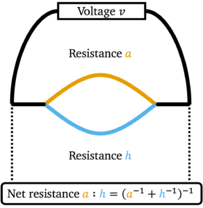
Let us put aside the randomized SVD for a moment and digress to the seemingly unrelated topic of electrical circuits. Suppose we have a battery of voltage $v$ and we connect the ends using a wire of resistance $a$ . The current $\mathrm{curr}_a$ is given by Ohm’s law

$v = a \cdot \mathrm{curr}_a.$

Similarly, if the wire is replaced by a different wire with resistance $h$ , the current $\mathrm{curr}_h$ is then

$v = h \cdot \mathrm{curr}_h.$

Now comes the interesting question. What if we connect the battery by both wires (resistances $a$ and $h$ ) simultaneously in parallel, so that current can flow through either wire? Since wires of resistances $a$ and $h$ still have voltage $v$ , Ohm’s law still applies and thus the total current is

$\mathrm{curr}_{\rm total} = \mathrm{curr}_a + \mathrm{curr}_h = \frac{v}{a} + \frac{v}{h} = v \left(a^{-1}+h^{-1}\right).$

The net effect of connecting resisting wires of resistances $a$ and $h$ is the same as a single resisting wire of resistance

(8) $a:h \coloneqq \frac{v}{\mathrm{curr}_{\rm total}} = \left( a^{-1}+h^{-1}\right)^{-1}.$

We call the the operation $a \mathbin{:} h$ the parallel sum of $a$ and $h$ because it describes how resistances combine when connected in parallel.

The parallel sum operation $:$ can be extended to all nonnegative numbers $a$ and $h$ by continuity:

$a:h \coloneqq \lim_{b\downarrow a, \: k\downarrow h} b:k = \begin{cases}\left( a^{-1}+h^{-1}\right)^{-1}, & a,h > 0 ,\\0, & \textrm{otherwise}.\end{cases}$

Electrically, this definition states that one obtains a short circuit (resistance $0$ ) if either of the wires carries zero resistance.

Parallel sums of matrices were introduced by William N. Anderson, Jr. and Richard J. Duffin as a generalization of the parallel sum operation from electrical circuits. There are several equivalent definitions. The natural definition (8) applies for positive definite matrices

$A:H = (A^{-1}+H^{-1})^{-1} \quad \text{for $A,H$ positive definite.}$

This definition can be extended to positive semidefinite matrices by continuity. It can be useful to have an explicit definition which applies even to positive semidefinite matrices. To do so, observe that the (scalar) parallel sum satisfies the identity

$a:h = \frac{1}{a^{-1}+h^{-1}} = \frac{ah}{a+h} = \frac{a(a+h)-a^2}{a+h} = a - a(a+h)^{-1}a.$

To extend to matrices, we capitalize the letters and use the Moore–Penrose pseudoinverse in place of the inverse:

$A : H = A - A(A+H)^\dagger A.$

This was the definition (6) of the parallel sum we gave above which we found naturally in our randomized SVD error bounds.

The parallel sum enjoys a number of beautiful properties, some of which we list here:

Symmetry. $A:H = H:A$ ,
Simplified formula. $A:H = (A^{-1}+H^{-1})^{-1}$ for positive definite matrices,
Bounds. $A:H \preceq A$ and $A:H \preceq H$ .
Monotone. $A\mapsto (A:H)$ is monotone in the Loewner order.
Concavity. The map $(A,H) \mapsto A:H$ is (jointly) concave (with respect to the Loewner order).
Conjugation. For any square $C$ , $C^*(A:H)C = (C^*AC):(C^*HC)$ .
Trace. $\tr(A:H) \le (\tr A):(\tr H)$ .²
Unitarily invariant norms. $\left\|A:H\right\|_{\rm UI} \le \left\|A\right\|_{\rm UI} : \left\|H\right\|_{\rm UI}$ .

For completionists, we include a proof of the last property for reference.

Proof of Property 8

Let $\left\|\cdot\right\|_{\rm UI}'$ be the unitarily invariant norm dual to $\left\|\cdot\right\|_{\rm UI}$ .³ By duality, we have

$\begin{align*}\left\|A:H\right\|_{\rm UI} &= \max_{M\succeq 0,\: \left\|M\right\|_{\rm UI}'\le 1} \tr((A:H)M) \\&= \max_{M\succeq 0,\: \left\|M\right\|_{\rm UI}'\le 1} \tr(M^{1/2}(A:H)M^{1/2})\\&= \max_{M\succeq 0,\: \left\|M\right\|_{\rm UI}'\le 1} \tr((M^{1/2}AM^{1/2}):(M^{1/2}HM^{1/2})) \\&\le \max_{M\succeq 0,\: \left\|M\right\|_{\rm UI}'\le 1} \left[\tr(M^{1/2}AM^{1/2}):\tr(M^{1/2}HM^{1/2}) \right] \\&\le \left[\max_{M\succeq 0,\: \left\|M\right\|_{\rm UI}'\le 1} \tr(M^{1/2}AM^{1/2})\right]:\left[\max_{M\succeq 0,\: \left\|M\right\|_{\rm UI}'\le 1} \tr(M^{1/2}HM^{1/2})\right]\\&= \left\|A\right\|_{\rm UI} : \left\|H\right\|_{\rm UI}.\end{align*}$

The first line is duality, the second holds because $M\succeq 0$ , the third line is property 6, the fourth line is property 7, the fifth line is property 4, and the sixth line is duality.

Nearing the Finish: Enter the Randomness

Equipped with knowledge about parallel sums, we are now prepared to return to bounding the error of the randomized SVD. Apply property 8 of the parallel sum to the randomized SVD bound (7) to obtain

$\begin{align*}\left\|B - X\right\|_{\rm Q}^2&\le \left\| \Sigma_2 \right\|_{\rm Q}^2 + \left\|\Sigma_1^2 : [(\Sigma_2\Omega_2\Omega_1^\dagger)^*(\Sigma_2\Omega_2\Omega_1^\dagger)]\right\|_{\rm UI} \\&\le \left\| \Sigma_2 \right\|_{\rm Q}^2 + \left\|\Sigma_1^2\right\|_{\rm UI} : \left\|[(\Sigma_2\Omega_2\Omega_1^\dagger)^*(\Sigma_2\Omega_2\Omega_1^\dagger)]\right\|_{\rm UI} \\&= \left\| \Sigma_2 \right\|_{\rm Q}^2 + \left\|\Sigma_1\right\|_{\rm Q}^2 : \left\|\Sigma_2\Omega_2\Omega_1^\dagger\right\|^2_{\rm Q}.\end{align*}$

This bound is totally deterministic: It holds for any choice of test matrix $\Omega$ , random or otherwise. We can use this bound to analyze the randomized SVD in many different ways for different kinds of random (or non-random) matrices $\Omega$ . Tropp and Webber provide a number of examples instantiating this general bound in different ways.

We shall present only the simplest error bound for randomized SVD. We make the following assumptions:

The test matrix $\Omega$ is standard Gaussian.⁴
The norm $\left\|\cdot\right\|_{\rm Q}$ is the Frobenius norm $\left\|\cdot\right\|_{\rm F}$ .
The randomized SVD rank $k$ is $\ge r-2$ .

Under these assumptions and using the property $a : h \le h$ , we obtain the following expression for the expected error of the randomized SVD

(9) $\mathbb{E} \left\|B - X\right\|_{\rm F}^2\le \left\| B - \lowrank{B\right\|_r }_{\rm F}^2 + \mathbb{E}\left\|\Sigma_2\Omega_2\Omega_1^\dagger\right\|^2_{\rm F}.$

All that is left to is compute the expectation of $\left\|\Sigma_2\Omega_2\Omega_1^\dagger\right\|_{\rm F}^2$ . Remarkably, this can be done in closed form.

Aside: Expectation of Gaussian–Inverse Gaussian Matrix Product

The final ingredient in our randomized SVD analysis is the following computation involving Gaussian random matrices. Let $G$ and $\Gamma$ be independent standard Gaussian random matrices with $\Gamma$ of size $r\times k$ , $k\ge r-2$ . Then

$\mathbb{E} \left\|SG\Gamma^\dagger R\right\|_{\rm F}^2 = \frac{1}{k-(r+1)}\left\|S\right\|_{\rm F}^2\left\|R\right\|_{\rm F}^2.$

For the probability lovers, we will now go on to prove this. For those who are less probabilistically inclined, this result can be treated as a black box.

Proof of Random Matrix Formula

To prove this, first consider a simpler case where $\Gamma^\dagger$ does not appear:

$\mathbb{E} \left\|SGW\right\|_{\rm F}^2 = \mathbb{E} \sum_{ij} \left(\sum_{k\ell} s_{ik}g_{k\ell}w_{\ell j} \right)^2 = \mathbb{E} \sum_{ijk\ell} s_{ik}^2 w_{\ell j}^2 = \left\|S\right\|_{\rm F}^2\left\|W\right\|_{\rm F}^2.$

Here, we used the fact that the entries $g_{k\ell}$ are independent, mean-zero, and variance-one. Thus, applying this result conditionally on $\Gamma$ with $W = \Gamma^\dagger R$ , we get

(10) $\mathbb{E} \left\|SG\Gamma^\dagger R\right\|_{\rm F}^2 =\mathbb{E}\left[ \mathbb{E}\left[ \left\|SG\Gamma^\dagger R\right\|_{\rm F}^2 \,\middle|\, \Gamma\right]\right] =\left\|S\right\|_{\rm F}^2\cdot \mathbb{E} \left\|\Gamma^\dagger R\right\|_{\rm F}^2.$

To compute $\mathbb{E} \left\|\Gamma^\dagger R\right\|_{\rm F}^2$ , we rewrite using the trace

$\mathbb{E} \left\|\Gamma^\dagger R\right\|_{\rm F}^2 = \mathbb{E} \tr \left(\Gamma^\dagger RR^* \Gamma^{*\dagger} \right)= \tr \left(RR^* \mathbb{E}[\Gamma^{*\dagger}\Gamma^\dagger] \right) = \tr \left(RR^* \mathbb{E}[(\Gamma\Gamma^*)^{-1}] \right).$

The matrix $(\Gamma\Gamma^*)^{-1}$ is known as an inverse-Wishart matrix and is a well-studied random matrix model. In particular, its expectation is known to be $(k-(r+1))^{-1}I$ . Thus, we obtain

$\mathbb{E} \left\|\Gamma^\dagger R\right\|_{\rm F}^2 = \tr \left(RR^* \mathbb{E}[(\Gamma\Gamma^*)^{-1}] \right) = \frac{\tr \left(RR^* \right)}{k-(r+1)} = \frac{\left\|R\right\|_{\rm F}^2}{k-(r+1)}.$

Plugging into (10), we obtain the desired conclusion

$\mathbb{E} \left\|SG\Gamma^\dagger R\right\|_{\rm F}^2 =\left\|S\right\|_{\rm F}^2\cdot \mathbb{E} \left\|\Gamma^\dagger R\right\|_{\rm F}^2 = \frac{1}{k-(r+1)}\left\|S\right\|_{\rm F}^2\left\|R\right\|_{\rm F}^2.$

This completes the proof.

Wrapping it All Up

We’re now within striking distance. All that is left is to assemble the pieces we have been working with to obtain a final bound for the randomized SVD.

Recall we have chosen the random matrix $\Omega$ to be standard Gaussian. By the rotational invariance of the Gaussian distribution, $\Omega_1$ and $\Omega_2$ are independent and standard Gaussian as well. Plugging the matrix expectation bound to (9) then completes the analysis

$\begin{align*}\mathbb{E} \left\|B - X\right\|_{\rm F}^2&\le \left\| B - \lowrank{B\right\|_r }_{\rm F}^2 + \mathbb{E}\norm{\Sigma_2\Omega_2\Omega_1^\dagger I_{k\times k}}^2_{\rm F} \\&= \left\| B - \lowrank{B\right\|_r }_{\rm F}^2 + \frac{\left\|\Sigma_2\right\|_{\rm F}^2\norm{I_{k\times k}}_{\rm F}^2}{k-(r+1)} \\&= \left(1 + \frac{k}{k-(r+1)}\right) \left\| B - \lowrank{B\right\|_r }_{\rm F}^2.\end{align*}$